The hidden sunrise in the energy-energy correlator (collider physics)
The content on this page was written by AI under human supervision.
The energy–energy correlator, one of the few collider measurements that can be computed exactly order by order, describes how the energy of a collision is shared between pairs of directions a given angle apart. In the supersymmetric cousin of quantum chromodynamics (QCD) that theorists use as a proving ground, its third-order prediction had been known since 2019 except for one two-fold integral that had resisted evaluation. The paper summarized here evaluates that integral in closed form by showing that it lives on the elliptic curve of the sunrise diagram, the first Feynman integral known to require elliptic functions.
Energy flow at a fixed angle
When an electron and a positron annihilate at high energy, a spray of particles comes out in all directions. In the late 1970s Basham, Brown, Ellis and Love proposed a simple summary of such an event: take every pair of outgoing particles, weight the pair by the product of its two energies, and record the angle $\chi$ between them. Averaged over many collisions this gives a distribution in the angle, the energy–energy correlator or EEC. As an energy-weighted cross section,
$$\frac{d\sigma}{d\zeta}= \sum_{ij}\int d\text{LIPS}\; |\mathcal{M}|^2 \,\frac{E_iE_j}{Q^2}\; \delta\!\left(\zeta-\frac{1-\cos\theta_{ij}}{2}\right).$$The sum runs over all pairs of final-state particles $i$ and $j$, with energies $E_i$, $E_j$ and relative angle $\theta_{ij}$; $Q$ is the total collision energy, $|\mathcal{M}|^2$ the squared quantum amplitude for that final state, and $d\text{LIPS}$ the integration over all allowed final-state momenta. The delta function keeps only pairs at the chosen angle, which the paper trades for the variable $\zeta=(1-\cos\chi)/2$ running from 0 to 1. Nearly parallel pairs give $\zeta\to0$, the collinear limit; opposite pairs give $\zeta\to1$, the back-to-back limit.
The EEC is, in the paper’s words, among the simplest observables in perturbative QCD, the theory of quarks and gluons. It is infrared finite, needs no jet algorithm, compares directly with data, and has been used to measure the strong coupling. That simplicity also lets one study what kinds of functions a physical measurement is made of.
Exact results before this work
Predictions for the EEC come as a series in the coupling strength: leading order (LO), next-to-leading order (NLO), next-to-next-to-leading order (NNLO), each harder than the last. Alongside QCD, theorists work in $\mathcal{N}=4$ super-Yang–Mills theory, a far more symmetric relative that shares many perturbative features with QCD and serves as a simpler model for developing techniques. In QCD the EEC is known analytically through NLO, for electron–positron annihilation (2018) and for Higgs-boson decays to hadrons (2019–2021). In $\mathcal{N}=4$ it is known one order further: at NLO since 2014, and at NNLO since the 2019 calculation of Henn, Sokatchev, Yan and Zhiboedov, the paper’s reference [1].
All the exact results through NLO are polylogarithmsThe logarithm, the dilogarithm $\mathrm{Li}_2$ and their generalizations: functions built by repeatedly integrating simple rational forms, one integration inside the next. The number of nested integrations is the weight; $\log$ has weight one, $\pi^2$ and $\mathrm{Li}_2$ weight two, $\zeta_3$ weight three. of weight up to three, a class with a well-developed algebra and public programs that evaluate its members fast and to high precision. The 2019 NNLO result almost fits in the same class. Its authors reduced the answer to harmonic polylogarithms of weight up to five plus one leftover: a finite two-fold integral of a rational kernel multiplying weight-three polylogarithms, left unevaluated. They also observed that the kernel is tied to the elliptic curve of the equal-mass sunrise integral. That leftover, $F_R(\zeta)$ in the paper’s notation, is the integral the present paper evaluates.
When polylogarithms run out
An integral stays polylogarithmic as long as every square root in its integrand can be removed by a change of variables. The square root of a quadratic polynomial always can be. The square root of a cubic or quartic $Q(x)$ with distinct roots cannot, and the equation $y^2=Q(x)$ then defines a new geometric object, an elliptic curveThe set of solutions of $y^2=Q(x)$ with $Q$ a cubic or quartic polynomial. Over the complex numbers its points form a surface with one hole, a torus. Integrals around the two independent cycles of the torus are its periods, the complete elliptic integrals; as the curve’s parameter varies they obey a second-order differential equation called the Picard–Fuchs equation.. Its basic integrals are elliptic integrals rather than logarithms, and functions built on top of them lie outside the polylogarithms, where the tools are far less developed. The authors note in their introduction that, for energy correlators, elliptic functions first appear in the EEC at NNLO and in the four-point correlator at LO, the latter treated on its own page, the four-point correlator.
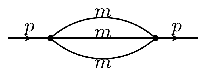
The sunrise diagram. A particle of momentum $p$ turns into three virtual particles of the same mass $m$, which recombine. Taken in two dimensions, as the paper does, the corresponding two-loop integral is finite and depends only on the ratio $S/m^2$ with $S=p^2$; it is the first Feynman integral known to require elliptic functions. (The diagram as drawn in Eq. (23) of the paper.)
The two-loop sunrise diagram with three equal masses, drawn above, has been studied extensively; the paper cites Laporta and Remiddi, Adams, Bogner and Weinzierl, and Bloch and Vanhove, among others. Writing it in Feynman parameters and completing a square exposes the square root of a quartic, which defines the sunrise curve. As the invariant mass $S=p^2$ flowing through the diagram varies, the curve changes shape, and it degenerates at exactly four values, $S/m^2=0,\,1,\,9,\,\infty$; the value $9m^2=(3m)^2$ is the threshold at which the three internal particles can all become real. All four degenerations are of one particular kind (the technical term is maximally unipotent), which makes the family special. The sunrise family is governed by a subgroup of the modular group called $\Gamma_1(6)$, whose natural functions are modular formsA torus is described, up to rescaling, by one complex number $\tau$, and changing $\tau$ by an element of the modular group $\mathrm{SL}(2,\mathbb{Z})$ gives back the same torus. Modular forms are functions of $\tau$ that transform in a prescribed way under the modular group or one of its subgroups, such as $\Gamma_1(6)$; they have power-series expansions in $q=e^{2\pi i\tau}$ with highly structured coefficients; the simplest examples are the Eisenstein series. The four degeneration points of the sunrise family are the four cusps of $\Gamma_1(6)$.. Work since the mid-2000s has made the sunrise’s periods, its modular parametrization and the iterated integrals of its modular forms explicit.
The same curve as the sunrise diagram
The paper first reorganizes $F_R$. Its kernel involves three quadratic polynomials in the inner integration variable $x$; one factors and yields only logarithms, while the other two, $D_1$ and $D_2$, have discriminants that are not perfect squares and are the source of everything elliptic. A partial-fraction decomposition, organized by what the paper calls the Galois symmetry of the integrand (flipping the sign of either square root must change nothing), splits $F_R$ into three finite pieces: $F_{{\rm red}_1}$, free of square roots and therefore polylogarithmic, and two irreducible pieces $F_{K_1}$ and $F_{R_2}$ with one square root each. After the $x$ integration, the expression under each square root is a quartic in the outer variable $\bar z$. The first defines the curve
$$\mathcal{C}_\zeta:\qquad y^2\;=\;Q_1(\bar z)\;=\;\left(\bar z^{\,2}-\bar z+2\zeta^2-\zeta\right)^2+4\,\zeta^3(1-\zeta).$$Each angle $\zeta$ thus comes with its own elliptic curve. Written this way $Q_1$ is a square plus a positive number whenever $0\lt\zeta\lt1$, so the integrand is real across the physical range, with all of its singularities on the boundary of the integration region. The second quartic, $Q_2$, looks different, but the Möbius map $w=\bar z/(\bar z-1)$ gives $Q_2(\bar z)=(\bar z-1)^4\,Q_1(w)$ and carries the integration measure of $F_{R_2}$ into that of $F_{K_1}$. The two irreducible pieces are integrals over one and the same curve along different paths. The coordinate-independent test of whether two elliptic curves coincide is to compare their $j$-invariantsA single number computed from the coefficients of the cubic or quartic that defines an elliptic curve. Two curves can be carried into each other by a change of coordinates (over the complex numbers) exactly when their $j$-invariants are equal. For a family of curves depending on a parameter, $j$ is a rational function of that parameter whose poles mark where the curve degenerates.. For $\mathcal{C}_\zeta$ the paper finds
$$j(\zeta)\;=\;\frac{(1+2\zeta)^3\left(8\zeta^3-12\zeta^2+6\zeta+1\right)^3}{\zeta^6\,(1-\zeta)^2\,(1+8\zeta)}.$$The poles of $j(\zeta)$ sit at the collinear and back-to-back points $\zeta=0$ and $\zeta=1$, at infinity, and at one more finite point, $\zeta=-1/8$, which lies outside the physical range and looks accidental. The sunrise’s $j$-invariant is a rational function of $S/m^2$ with poles at its four degeneration points, and substituting $S=m^2(\zeta-1)/\zeta$ into it reproduces the expression above identically in $\zeta$. The special points match one to one, $S/m^2=\infty,\,0,\,9,\,1$ against $\zeta=0,\,1,\,-1/8,\,\infty$, so the puzzling $\zeta=-1/8$ corresponds to the three-particle threshold $S=9m^2$. Physical angles map to negative $S/m^2$, the Euclidean region of the sunrise below every threshold, which is why nothing singular happens between the collinear limit at $S\to-\infty$ and the back-to-back limit at $S\to0$.
Sharing a curve does not make two integrals equal, and the authors determine how the two are related using differential equations. Differentiating $F_{K_1}$ twice in $\zeta$ produces one new two-fold integral, $S_0(\zeta)$, and the pair closes into a second-order system. The system is built on the sunrise’s Picard–Fuchs operator, $\zeta(\zeta-1)(8\zeta+1)\,\partial_\zeta^2+(24\zeta^2-14\zeta-1)\,\partial_\zeta+2(4\zeta-1)$, with $\partial_\zeta$ the derivative in $\zeta$. Because the system is second order, no geometry beyond an elliptic curve can appear. Running the same analysis on $F_{R_2}$ and subtracting shows that $\Delta=F_{R_2}-F_{K_1}$ is itself a polylogarithm, given in closed form. So $F_R=2F_{K_1}+P(\zeta)$ with $P$ polylogarithmic, and one elliptic function remains to be found.
The finished formula
The polylogarithmic part $P(\zeta)$ comes from doing both integrations directly with HyperInt, Erik Panzer’s program for such integrals. It fills about a page: harmonic polylogarithms of weight up to five whose letters (the elementary arguments fed into the nested integrations) are only $\zeta$ and $1-\zeta$, with rational-function coefficients and the constants $\pi^2$, $\zeta_3$, $\pi^4$, $\zeta_5$ and $\pi^2\zeta_3$.
The elliptic part is solved in what the paper calls the modular frame. The Picard–Fuchs operator has a power-series solution at the collinear point, the period $\psi_1(\zeta)=1-2\zeta+10\zeta^2-56\zeta^3+\dots$, whose coefficients are, up to sign, the Franel numbers $\sum_k\binom{n}{k}^3$. Exponentiating the ratio of its two solutions gives a new variable $q=\zeta-3\zeta^2+15\zeta^3-\dots$, and conversely $\zeta$ and $\psi_1$ are modular objects for $\Gamma_1(6)$, quotients of Dedekind eta functions. In this frame the equation for $S_0$ becomes two successive integrations in $\log q$, and the answer is a combination of iterated integrals $I(f_1,\dots,f_n;q)$ whose kernels $f_i$ are modular forms, the paper’s iterated Eisenstein integrals. Apart from a trivial constant kernel, only four occur: $d\log\zeta$ and $-d\log(1-\zeta)$ rewritten in $q$, called $\omega_0$ and $\omega_1$, which the polylogarithms already use, and two new ones of modular weight three, $\psi_1\omega_0$ and $\zeta\psi_1\omega_0$, through which the curve enters. The function $S_0/\psi_1$ comes out as three boundary terms plus thirteen such iterated integrals of length up to five, each with a rational coefficient, in a few cases times $\pi^2$ or $\zeta_3$ (Eq. (61) of the paper).
The complete correlator is then $F_{\rm NNLO}=F_{\rm P}+F_{\rm E}$. Here $F_{\rm P}$ gathers all the harmonic polylogarithms, of argument $\sqrt{\zeta}$ and weight up to five. The elliptic part is $F_{\rm E}=2A\,S_0/\psi_1+2B\,\theta(S_0/\psi_1)$, with $\theta=q\,d/dq$ and coefficients $A$ and $B$ built from rational functions of $\zeta$, the period $\psi_1$ and its derivative. Every ingredient is explicit and cheap to evaluate: find the $q_0$ for the chosen angle, expand the kernels as integer $q$-series, and build the iterated integrals from the inside out as truncated series with rational coefficients, rounding only at the end. The number of correct digits grows linearly with the truncation order $N$, roughly as $D\simeq N\log_{10}(1/q_0)-3$; fifty digits take about 75 terms at $\zeta_0=3/11$ and about 106 at $\zeta_0=1/2$. This truncated-series method is the standard one for iterated integrals of modular forms and is also implemented in the GiNaC library, against which the authors checked their own implementation. With it the NNLO distribution comes out to high precision within seconds.
Checks at the two ends
The paper expands the closed form to third order at both ends of the angular range. In the collinear limit the expansion begins $\zeta\left[\tfrac12\log^2\zeta+\left(-5+\tfrac{\pi^2}{3}-\zeta_3\right)\log\zeta+\dots\right]$, and every constant in it is a zeta value. The back-to-back expansion begins $-\tfrac18\log^5(1-\zeta)$; its subleading terms need $\log2$, polylogarithms at one half, and one new constant, $S_0(1)\approx13.8046$, the elliptic function at the second cusp, which involves a sixth root of unity. In each limit the leading terms are fixed independently by a general theory of that limit: the light-ray operator product expansion on the collinear side and Sudakov resummation on the back-to-back side.
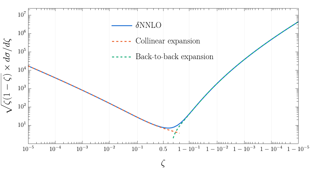
The pure third-order term of the correlator (solid blue, labeled $\delta$NNLO), multiplied by $\sqrt{\zeta(1-\zeta)}$ and drawn against $\zeta$ on an axis stretched logarithmically toward both endpoints, together with its collinear expansion through order $\zeta^3$ (orange dashed) and its back-to-back expansion through order $(1-\zeta)^2$ (green dashed). Each expansion tracks the exact curve over many decades on its own side, and the collinear one remains reliable out to $\zeta\approx0.5$. (Figure 1 of the paper.)
The first figure shows the pure NNLO term together with both expansions across ten decades of the stretched $\zeta$ axis; each series hugs the exact curve on its own side. The second plots the correlator summed through LO, NLO and NNLO at a sample coupling. In the bulk of the range the orders sit close together and fixed order is reliable. Toward either endpoint large logarithms of $\zeta$ or $1-\zeta$ take over, the orders pull apart, and the NLO curve even turns negative near $1-\zeta\sim10^{-2}$. There the logarithms must be resummed to all orders, which for the EEC has been done to high accuracy in both limits; fixed-order results such as this one supply the ingredients.
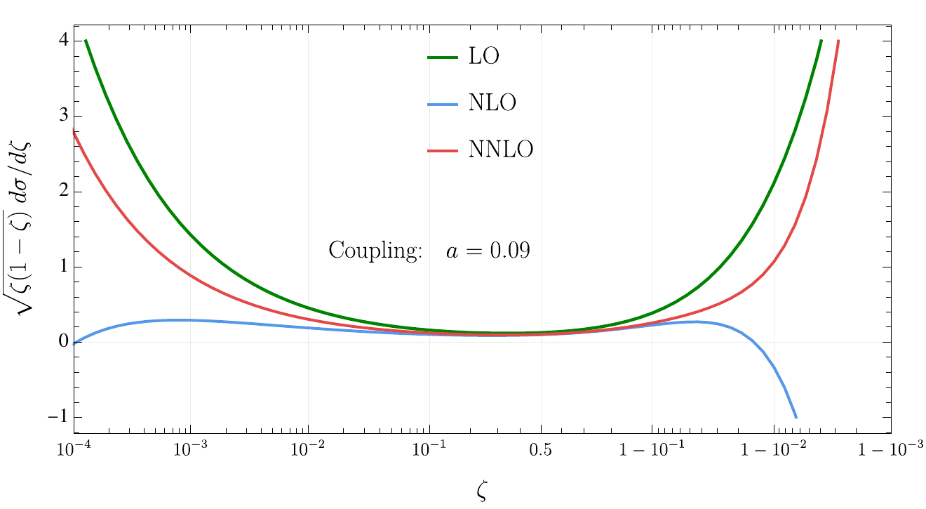
The correlator in $\mathcal{N}=4$ super-Yang–Mills at leading order (green), through NLO (blue) and through NNLO (red), for a sample coupling $a=0.09$, multiplied by $\sqrt{\zeta(1-\zeta)}$ and drawn on the same stretched axis. The orders converge well in the bulk; near both endpoints large logarithms make them disagree, and the NLO curve goes negative near $1-\zeta\sim10^{-2}$, so resummation is required there. (Figure 2 of the paper.)
A first look at a bootstrap, and the outlook for QCD
With the closed form known, the authors ask how much of it could have been written down without doing the integrals, from the possible singularities, the curve and the known limits alone. Such bootstraps have fixed whole scattering amplitudes in planar $\mathcal{N}=4$, where the unknown coefficients are pure numbers; here they are rational functions of $\zeta$, and far more numerous. The polylogarithmic letters, derived from the integrand, are $\zeta$, $1-\zeta$ and $(1-\sqrt{\zeta})/(1+\sqrt{\zeta})$; on the elliptic side the curve, its Picard–Fuchs operator and the positions of the physical singularities allow only six kernels, so the space of candidate functions is finite, which the paper stresses is far from automatic. At NLO the ansatz has 206 rational parameters, and 76 of them are fixed by physical requirements: regularity at the endpoints, the known leading terms, a sum rule. The other 130 are fixed by fitting 126 high-precision values, and the result agrees term by term with the 2014 calculation. At NNLO the joint ansatz has 2336 parameters, and as a robustness test its elliptic part is written without assuming in advance which six kernels are allowed. The physical requirements fix 373, merging parameters that enter only in fixed combinations removes 113 more, and the remaining 1850 are recovered in one step by lattice reduction, an integer-relation method, run with the program Flatter. That step succeeds from 150 values at 350 digits (119.5 CPU hours), and equally from 300 values at 270 digits, 600 at 225 or 1200 at 205 (50.4, 56.1 and 62.1 CPU hours). The recovered answer uses only the six kernels. With more sample points fewer digits per point are needed, but the authors estimate that this gain levels off near 200 digits per point, and that at 100 digits or fewer no number of points up to 2400 would suffice.
The paper’s first caveat about the bootstrap is that the numerical values were generated from the analytic result itself rather than from an independent high-precision evaluator of the EEC, which a real bootstrap would need. Its second is that physical constraints alone fixed only 16% of the NNLO parameters, with about 80% coming from the numerical data, so either new consistency conditions must be found or precise numerics must carry most of the load, as they could here.
The authors are cautious about what the result implies for QCD. The elliptic function space here was fixed by geometry, the curve and its level, rather than by anything specific to the supersymmetric theory, and the curve follows from the integrand alone. The QCD integrand at this order is known even though its integrals are not. The paper suggests that the same analysis would identify its elliptic letters and function space in advance and could bypass steps of a direct calculation. It calls a complete bootstrap of the NNLO correlator in QCD difficult. The numerical method carries over directly: a QCD result written in iterated Eisenstein integrals would be just as fast to evaluate, at the precision collider studies need.
The paper
- The hidden sunrise in the energy-energy correlator (PDF) — Matthew D. Schwartz and Xiaoyuan Zhang; the source of everything above. Evaluates in closed form the two-fold integral left over from the 2019 NNLO calculation of the correlator in $\mathcal{N}=4$ super-Yang–Mills theory, in harmonic polylogarithms and iterated Eisenstein integrals on the sunrise curve, with a fast numerical evaluator, expansions at both ends of the angular range and a first bootstrap study; the authors write out every formula in full, down to the source terms of the differential system in an appendix.
The overview and the companion four-point work are on the Energy correlators page and the four-point page.
Supplementary material
Five files accompany this page, all using an equivalent representation of their own: a finite sum of one-fold integrals over the sunrise curve with exact coefficients rather than $q$-series. Each evaluator compares its output with direct numerical integration of the defining two-fold integrals as it runs. The header of each script documents its interface; at default settings the scripts finish within a few minutes on one core.
- fk1-evaluate.py — Python (mpmath): evaluates the elliptic piece $F_{K_1}$ at a rational angle $\zeta$ between $1/10$ and $3/4$, to a requested number of digits, from the coefficient table in fk1_words.json, and checks the decoded coefficients against direct quadrature of the defining $K_1$ integrand on every run. A slower
--deepmode recomputes $F_{K_1}$ independently by solving the pulled-back sunrise differential equation. - fell-evaluate.py — Python (mpmath): evaluates the complete remainder $F_R=F_{K_1}+F_{R_2}+F_{{\rm red}_1}$, with $F_{K_1}$ from the same coefficient table, $F_{R_2}$ as a one-fold integral over the same curve after the Möbius map, and $F_{{\rm red}_1}$ from its representation in polylogarithms.
- fk1_words.json — the coefficient table for $F_{K_1}$: its 159 one-fold integrals over the sunrise curve and their exact coefficients, none fitted. Required by both evaluators, which check its SHA-256 digest when they load it.
- fr2_words.json — the coefficient table for $F_{R_2}$ in the same representation: 578 terms with exact coefficients, none fitted.
- fell_symbolic.py — the same mathematics as sympy expressions with an mpmath quadrature layer: the sunrise quartic, the symbolic forms of all three pieces, the 159-term table for $F_{K_1}$ and the exact 112-term polylogarithm expansion of the inner integral of $F_{{\rm red}_1}$.
python3 fell_symbolic.py --selftestproves the exact identities of the rational layer symbolically, matches the $F_{K_1}$ table against fk1_words.json and the $F_{{\rm red}_1}$ table against the copy inside fell-evaluate.py, and evaluates the three pieces and their sum at $\zeta=1/3$ and $1/2$ against fell-evaluate.py.
References
| C. L. Basham, L. S. Brown, S. D. Ellis and S. T. Love, Energy correlations in electron-positron annihilation: testing QCD, Phys. Rev. Lett. 41 (1978) 1585 | proposed the energy–energy correlator as a test of QCD |
| A. V. Belitsky, S. Hohenegger, G. P. Korchemsky, E. Sokatchev and A. Zhiboedov, Energy-energy correlations in $\mathcal{N}=4$ supersymmetric Yang–Mills theory, Phys. Rev. Lett. 112 (2014) 071601 | the NLO correlator in $\mathcal{N}=4$, which the NLO bootstrap test reproduces term by term |
| L. J. Dixon, M.-X. Luo, V. Shtabovenko, T.-Z. Yang and H. X. Zhu, Analytical computation of energy-energy correlation at next-to-leading order in QCD, Phys. Rev. Lett. 120 (2018) 102001 | the analytic NLO correlator in QCD for electron–positron annihilation |
| M.-X. Luo, V. Shtabovenko, T.-Z. Yang and H. X. Zhu, Analytic next-to-leading order calculation of energy-energy correlation in gluon-initiated Higgs decays, JHEP 06 (2019) 037 | the analytic NLO correlator for Higgs-boson decays to gluons |
| J. Gao, V. Shtabovenko and T.-Z. Yang, Energy-energy correlation in hadronic Higgs decays: analytic results and phenomenology at NLO, JHEP 02 (2021) 210 | the analytic NLO correlator for Higgs-boson decays to hadrons, the 2021 result mentioned above |
| J. M. Henn, E. Sokatchev, K. Yan and A. Zhiboedov, Energy-energy correlation in $\mathcal{N}=4$ super Yang–Mills theory at next-to-next-to-leading order, Phys. Rev. D 100 (2019) 036010 | the NNLO correlator with one two-fold integral left unevaluated; the starting point |
| A. Sabry, Fourth order spectral functions for the electron propagator, Nucl. Phys. 33 (1962) 401 | where the equal-mass sunrise integral, and with it elliptic integrals, first entered a Feynman-diagram calculation |
| S. Laporta and E. Remiddi, Analytic treatment of the two loop equal mass sunrise graph, Nucl. Phys. B 704 (2005) 349 | the differential equation and analytic treatment of the equal-mass sunrise |
| L. Adams, C. Bogner and S. Weinzierl, The two-loop sunrise graph with arbitrary masses, J. Math. Phys. 54 (2013) 052303 | the sunrise in two dimensions for arbitrary masses, solved through its second-order differential equation |
| S. Bloch and P. Vanhove, The elliptic dilogarithm for the sunset graph, J. Number Theor. 148 (2015) 328 | the equal-mass sunrise as an elliptic dilogarithm and its $\Gamma_1(6)$ modular structure |
| L. Adams and S. Weinzierl, Feynman integrals and iterated integrals of modular forms, Commun. Num. Theor. Phys. 12 (2018) 193 | the sunrise family in iterated integrals of modular forms, the function class of the elliptic part |
| M. Walden and S. Weinzierl, Numerical evaluation of iterated integrals related to elliptic Feynman integrals, Comput. Phys. Commun. 265 (2021) 108020 | the truncated-series evaluation of such iterated integrals in GiNaC, against which the authors checked their implementation |
| E. Panzer, Algorithms for the symbolic integration of hyperlogarithms with applications to Feynman integrals, Comput. Phys. Commun. 188 (2015) 148 | the program HyperInt, used for the polylogarithmic part |
| D. Chicherin, J. Henn and V. Mitev, Bootstrapping pentagon functions, JHEP 05 (2018) 164 | one of the Landau (Feynman-integral) bootstrap calculations the introduction cites, the approach the paper’s own bootstrap study follows |
| O. Barrera, A. Dersy, R. Husain, M. D. Schwartz and X. Zhang, Analytic regression of Feynman integrals from high-precision numerical sampling, arXiv:2507.17815 (2025) | lattice reduction from numerical samples, the method of the bootstrap test |
| K. Ryan and N. Heninger, Fast practical lattice reduction through iterated compression, in Advances in Cryptology – CRYPTO 2023, Lecture Notes in Computer Science (Springer, 2023) 3 | the lattice-reduction program Flatter, used to recover the NNLO coefficients |