The BootLoops harness
A harness is an interface between a human user and a Large Language Model. There are many open source and commercial harnesses that effectively coerce functionality out of the models so you don't have to do it directly. BootLoops is a harness for precision quantitative science. It is essentially an extensive scientific software package ported or written by LLMs, and meant to be used by LLMs, supplemented by a set of guiding protocols that lets the LLM use the software more effectively. The harness is, by design, independent of the language model driving it. The BootLoops harness is entirely open-source, hosted on GitHub in a public repo, and can be cloned and used by anyone with any LLM. It is most efficiently used from a Command-Line-Interface (CLI) session that can run the code, but it can also be used through the Codex or Claude apps.
The BootLoops harness is essentially a toolkit — a repository of reduction engines, singularity finders, transport machinery, high-precision evaluators, integer-relation closersprograms that take a number known to hundreds of digits and find the exact combination of known constants it equals — small integer coefficients times $\pi$, $\zeta(3)$, and friends, certified-statistics packages — with each tool tested, documented on its own page, and wrapped in the conventions an LLM needs to drive it: what the instrument does, when to reach for it, what its output means, and what test its answer has to pass before anyone believes it. Some of the tools are mature community engines, adopted as-is or through a port; the rest were written inside the program, usually in the middle of a calculation, when nothing public covered the need.
The harness is also not a static object. The original toolkit BootLoops 1.0 was grown from the seed for one project to tools relevant for hundreds. When a problem demands something beyond the current tools' capabilities, rather than just trying to solve the problem by brute force, the idea is to search for what public tools exist that could help or whether the LLM could build a new tool on its own. Then the agent writes or upgrades the tools, tests it on cases with known answers, and files it to the harness. Then the next problem will have this banked and can start on the followup tools. None of this tooling depends on which model is driving. Importantly, the gains sit in the harness tools and their documentation, so any LLM, present or future, can pick them up. Anyone can build and improve their own local version of BootLoops, starting from the public repo and growing it for their applications. New additions can be submitted through pull requests so they can be validated and added to the toolkit for others to use.
The recommended use of the tool is as follows. Say you are interested in an integral you haven't been able to compute, or don't know if you can trust a Bayesian evidencethe total probability a model assigns to the observed data, averaged over all its parameter values — the number Bayesian statistics uses to compare models calculation you did, or want to know if there is an alternative to Monte Carlo sampling that will be more efficient than what you are doing. Whatever your problem is, you then ask your LLM: could BootLoops help with this problem? If you have the repo cloned locally (recommended, see below), it will search through existing tools to see if one applies and tell you the recommended path, or else search broadly for relevant tools or papers describing methods for tools that it could port or build to help. Or maybe your problem is just not BootLoops-shaped and it will tell you that. After that you work with the LLM to solve your problem.
The rest of this page is practical: it describes the tools and protocols currently in the harness (BootLoops 1.0). Then it describes some classes of problems BootLoops is good at — Feynman integrals and amplitudes, Bayesian evidence, certified arithmetic and audits, exhaustive enumeration and proof — each with the appropriate BootLoops standard its answers must meet. Installation options are given in Installation and the page ends with the human-intervention playbook: practical tips on succeeding at LLM-assisted science.
The toolkit
BootLoops comprises external and internal tools. The external tools are free-standing open-source projects it can clone and link to or tools that it ported from languages not well-suited to LLM use (Mathematica, MatLab, Stata, etc). Many of these it has upgraded: improved the numerical methods, added relevant subroutines, etc. Such upgrades are kept as forks: full copies of the upstream project carrying the BootLoops patches on top, separate from the originals so that the upstream code, license, and attribution stay intact and the patches can be offered back (e.g. the AMFlow fork in the repo's upgrades/). Most of the tools, however, Claude built on its own. Many of these are from ideas or algorithms from papers that were never made publicly available (e.g. Eichler, Leviathan, Landau Alphabet). Some are just creative ideas Claude had to build tools from scratch (e.g. Seedling, Mixalot).
Existing tools
public software, plugged in as-is or ported
New tools
written by Claude for BootLoops
Type size roughly tracks how many projects used the tool. Click any tool for the tool page to learn more about what the tool does and where it came from.
The tools all have their own pages describing what they do (click the tool name or use the Tool menu). Some tools have interesting origin stories. Consider for example:
- Eichler. Built to allow precision numerical evaluation of elliptic functions. It began with the Eichler integrals for the equal-mass sunrise, which Claude could not find any public package to compute. The next elliptic integral that came up sat on a different elliptic curvea curve cut out by $y^2=$ a cubic or quartic in $x$ — topologically a doughnut, and the simplest geometry whose integrals escape the logarithm family, so instead of adding one more function Claude generalized the library to the whole family, and the bananas then pushed it up to K3a four-dimensional geometry one rung above the elliptic curve, named for Kummer, Kähler, and Kodaira — home of the three-loop banana and Calabi–Yauthe higher-dimensional shapes string theory curls its extra dimensions into — and, it turns out, the natural geometry of four-loop banana diagrams periods. This powerful resulting library for period integrals was ideally suited for non-amplitudes projects, such as cosmological correlators, and period transport across the string-theory landscape.
- Baller. This is the ball-arithmetic package. The ball is an exact midpoint with a certified radius, so a computation with Baller propagates its own error bars as it runs. Baller uses Arb, a community C library, for the main hard work and packages instruments BootLoops built on top — certified quadraturenumerical integration — computing an integral by summing the integrand at carefully chosen points, certified transport, unique-zero proofs. The driver
baller.solveraises the working precision until the digits you asked for are certified. It will not hand back an uncertified answer by design; when a computation goes irrecoverably wrong — a divisor ball containing zero — the radius comes back infinite, so a wrong answer cannot be silently believed. It is used for the drug-trial reference values, the forest-census fit certificates — an interval-Newton step that turns a fitted optimum into a theorem — and the certified equilibria of the Great Oxidation model.
- Annihilator. Recovers, in exact arithmetic, the differential or recurrence operator a series is annihilated by and certifies that no lower-order operator exists. That certificate was used to refute the claim that the Watson integral factorizes: any candidate of a long-hunted closed form satisfies order 4, and the integral provably satisfies nothing below order 5. The same engine turns Bayesian evidence integrals into exact recurrences, and is used to fit recurrences in ecology, single-cell biology, mixtures, and linguistics.
- ERAS. Short for Exact Remainder-Aware Series, using Taylor expansions. Born from a spectacular failure of naive ball arithmetic: when a shared parameter enters every factor of a big product — a rate inside hundreds of per-observation terms — the intervals correlate nothing and the enclosure explodes (a measured width of 10²² on an integrand whose true sensitivity is a few hundred). ERAS restores usable certified widths with centered Taylor forms, classical validated numerics packaged with an adversarial verifier any adaptation must pass. It turned out to be the certified-arithmetic foundation of many applications: population genetics, trial designs, mixtures, and linguistics.
- Mixalot. Computes Bayesian evidence for mixture modelsstatistical models that read data as a blend of hidden subpopulations, each with its own distribution — the question is how many exactly. It builds on the same certified-integral machinery as the physics tools — Annihilator's exact recurrences and ERAS's certified arithmetic — to produce quantitatively precise Bayesian inference on how many parts something is made of, without restriction on the number of components or input complexity. Applications include looking for subpopulations on which a drug acts differently (the mixtures paper), authorship issues (which plays did Shakespeare have help with?), language history, and forest censuses in ecology.
- Numkin. This stands for numerical kinematics. It basically allows you to fit rational functions of multiple variables by plugging in rational numbers and solving. It was inspired by finite-field methodsdoing algebra with integers modulo a prime: every step exact, no rounding, and the true rational answer reconstructed at the end developed in computer algebra in the 1970s–80s (modular sampling, sparse rational interpolation) and brought into particle physics in the 2010s (see FireFly). Numkin chooses what to freeze and does a Thiele/Padé recombination with held-out certification. It powers a number of challenging geometric integrals (the anisotropic Watson integral). The same finite-field methodology enters the JaCK & Jill package (Jukes Cantor, Kimura + upgrades) used for Bayesian phylogenetics work: the contiguity recurrences in the evidence integrals are found and lifted mod-p and confirmed by rational reconstruction of the mod-p series.
- Wayfinder. It allows for the precision construction and evaluation of differential equations associated with iterated integrals. It first reconstructs a differential equation from a handful of numerical evaluations (plug in sample points, solve a linear system, and snap the entries exact with PSLQ) then it solves that equation outward from a boundary point to carry the answer anywhere in kinematic spacethe space of a process's physical inputs — energies, angles, masses — over which the answer is a function. It was inspired by the canonical-differential-equation program of Henn and the series-transport codes of particle physics (DiffExp, SeaSyde), but Claude wired the two halves into one instrument that checks itself: the reconstructed equation has to pass an exact flatness proof before it is trusted, and every transported value is checked against an independent evaluation at points never used in the fit. Wayfinder is the route for the sectors that value-fitting provably cannot reach — the Calabi–Yau banana block, the elliptic masters of gg→Zγ, and the elliptic sector of the nonplanar W-pair branch were closed this way.
Beyond the code: the protocol layer
Not everything in the harness is software. The repository ships a skills/ directory: the program's working protocols as standalone instruction files — plain markdown with a when-to-use header, readable by any model, so the harness stays model-independent in practice. To use one, point your agent at the file: "read skills/acceptance-gate/SKILL.md and hold my result to it."
Seven govern any quantitative work:
- acceptance-gate — what "done" means: a claimed answer reproduces an independent route at points never used in any fit, two-precision stable, with a positive control showing the check itself can fail.
- constant-recognition — integer-relation discipline: the candidate ringthe declared menu of constants — powers of $\pi$, $\zeta$-values, periods — a search may combine, fixed before looking so a match means something declared before the search, height boundscaps on how large the integers in a candidate relation may be — without them, some relation always "fits" any number, planted controls, and refusal over invention when nothing closes.
- planted-truth — every pipeline recovers a known, planted answer before touching real data, and deliberately corrupted inputs must be caught.
- independence-bookkeeping — provenance for every reference value; no <span class="def">oracle<span class="tip">an independent reference computation an answer is checked against — trustworthy only if it shared nothing with the fit it certifies</span></span> that fed a fit may certify the result.
- timing-discipline — measure a small run before launching a big one; a projection past a couple of hours calls for a smarter route, restructuring the problem rather than scaling the run.
- reading-contract — an instrument that reads documents asserts only what the record in front of it supports, citation attached; retrieval is never passed off as discovery.
- tool-stewardship — consult the toolkit before writing code, patch rather than fork, and document every new tool for the next agent: purpose, occasion, output, and the test its answer must pass.
One further protocol is enforced by the files themselves rather than by a skill: the verification substrate — integrity checkers and pinned reference bytes — is sha-pinned and fails closed if edited, and each such file opens with a plain do-not-edit notice aimed at the reader most likely to patch it: your agent. Everything else in the harness invites patching; the checkers do not.
Five carry heavier machinery for specific kinds of work:
- prove-protocol — proving with agents: an adversary hunts a counterexample before any proving starts, a hostile skeptic loop checks every step against executed exact scripts, independent provers run forced-distinct routes — and, when the statement itself is unknown or keeps dying, the theory-finding regime searches statement-space against an exact evaluator.
- referee-sim — before circulating any outward-facing document: simulate the strongest standard objection from every audience the document addresses, and verify it is answered where that reader would look.
- lit-review — the literature audit behind a novelty claim: every candidate paper read in full text rather than from memory, thoroughness made falsifiable through read ledgers and search receipts, citation chains chased in both directions.
- ref-check — bibliography verification against the authoritative databases, field by field, with the folklore-error traps that propagate through the literature.
- prose-lint — the machine-writing fingerprint, hunted before anything is published: banned vocabulary, banned sentence structures, agentless prose, and the honesty tells that matter most.
These protocols are as much a part of the harness as the code — an agent inherits them along with the ability to call the tools.
The toolkit at a glance
The packages sort into nine classes. A core of adopted community engines — Kira, AMFlow, PLD and SOFIA, pySecDec, and Arb among them — supplies the mature public machinery of multiloop computation. Everything else was written in the program. The complete index, one summary per package, is on the toolkit page.
Reduction engines. A two- or three-loop calculation opens with thousands of related integrals, sometimes millions, and integration-by-parts identities reduce them to a small independent basis. Kira, with FireFly and Fermat, is the adopted community workhorse; Blade, also adopted, was ported to run with no Mathematica underneath. Around them sit two tools BootLoops wrote: Seedling predicts what a reduction will cost before it is launched, and Winnow returns every identity with its own certificate.
Singularities and geometry. The bootstrappinning down an answer from its general properties — where it can blow up, what symmetries it obeys — instead of computing the integral head-on starts from where an integral can blow up. PLD and SOFIA, both adopted, compute the complete singular locus, certificate of completeness included; Leviathan is a clean-room reimplementation of the published Euler-characteristic-drop criterion for the same list, kept so the list is never computed only one way. GeoTriage then reads off which geometry the answer lives on — sphere, elliptic curve, K3, Calabi–Yau — and with it the class of functions to expect, and Maxcut computes the maximal cut that exposes that geometry.
Differential equations and transport. Exact answers travel: compute one point carefully, then carry it anywhere along the function's own differential equation. All four tools here are house-written. Counterweight rewrites a system into canonical form one exact balance at a time; Wayfinder reconstructs the equation from numerical samples of the connection and transports solutions along it; Vopclose closes graded systems layer by layer; and Annihilator recovers, in exact arithmetic, the differential or recurrence operator a series is annihilated by — including certified minimal order, the fact the Watson-integral impossibility proof rests on.
Evaluators and oracles. Every claimed formula is checked against numbers computed some other way, so the harness keeps several ways. AMFlow, adopted and extended, evaluates master integralsthe small independent set of integrals a calculation boils down to; every other integral in the problem is a combination of them to hundreds of digits by flowing in a fictitious mass; pySecDec and FIESTA, adopted, are kept exactly because they share no code with anything else in the harness. On the house side, Nestor is the quadrature oracle with certified error control, GPLEval is the polylogarithm evaluator behind the value-fits, and Eichler, written from scratch, covers elliptic and Calabi–Yau periods.
Closure and naming. A value computed to three hundred digits still needs a name. PSLQ is the adopted Ferguson–Bailey integer-relation algorithm, run under house discipline: height bounds, two-precision stability, planted controls. Lockpick brings heavier lattice machinery where plain PSLQ stalls and curates the ring of constants a search is allowed to draw on, so a null result means "not in this ring" rather than nothing; and Frobenius reaches boundary constants through arithmetic modulo primes, with no integration performed anywhere.
Certified arithmetic. The acceptance gates run on numbers that carry proofs of their own accuracy. Arb and mpmath, adopted, supply the substrate: every certified value is a midpoint with a rigorous radius around it. Baller packages the instruments the program built on top — certified quadrature, certified transport, unique-zero proofs — and ERAS restores usable error widths when a shared parameter makes naive ball arithmetic blow up.
Evidence and statistics. The same integral classes appear far from physics, and these packages, all house-written, apply the same certified standards there. Mixalot computes Bayesian evidence for mixture models exactly — the engine behind the forest-census and authorship results; Popcorn is the certified population-genetics toolbox behind the gnomAD analysis; JaCK & Jill delivers exact and certified evidence for phylogenetic trees, a tamper-evident certificate on every computation.
Enumeration and audits. Some questions are settled by counting everything. Terrier is the string-landscape suite — certified period transport and exact lattice arithmetic at census scale, every object in the census registered; Abacus counts the points of an abelian fourfold exactly from its period lattice alone; Qinvert works backward from published summary statistics to the smallest sets of data rows that reproduce them, in exact arithmetic.
Integrity. The last class keeps the other eight honest. Gatekeeper records the precision and provenance of every reference value and keeps independent oracles independent; Trust verifies reduction output through three checks with disjoint code lineages; Seedling’s family preflight checks an integral family’s symmetry and provenance before any reduction is launched, catching mislabeled topologies at the door.
The methods, by chapter. The main paper is organized around nine method families, each presented the same way: the characteristic problem, the integrals it handles, a worked example small enough to redo by hand, and where the corpus uses it. In the paper's order: integer-relation fits and constant recognition (PSLQ, Lockpick); holonomicsatisfying a linear differential or recurrence equation with polynomial coefficients — finite data that determines the function completely methods and creative telescopingan algorithm that mechanically finds the differential or recurrence equation an integral or sum obeys, certificate included (Annihilator); finite-field and multi-prime exact computer algebra (Kira/FireFly, Winnow); modular forms, periods, and arithmetic geometry (Eichler, Frobenius); exact ball arithmetic, certificates, and fail-closed computation (Baller, ERAS); lattice sums, exact enumeration, and dynamic programming (Terrier and the census engines); Bayesian evidence integrals (Mixalot, JaCK & Jill); calibrated inference against exact and planted truth (Popcorn); and LLM instruments with sources-only reading protocols (the reading-contract discipline). The five-step recipe in the amplitudes section below is the loop-integral entry point into that toolbox; the chapters are the toolbox itself.
Computing Feynman integrals and amplitudes
The loop integrals of quantum field theory are the use case the harness grew up on, and the one its deepest machinery serves: evaluate them exactly, by bootstrap where possible and by direct methods where needed, and hold every answer to a standard a machine can check.
The problem class
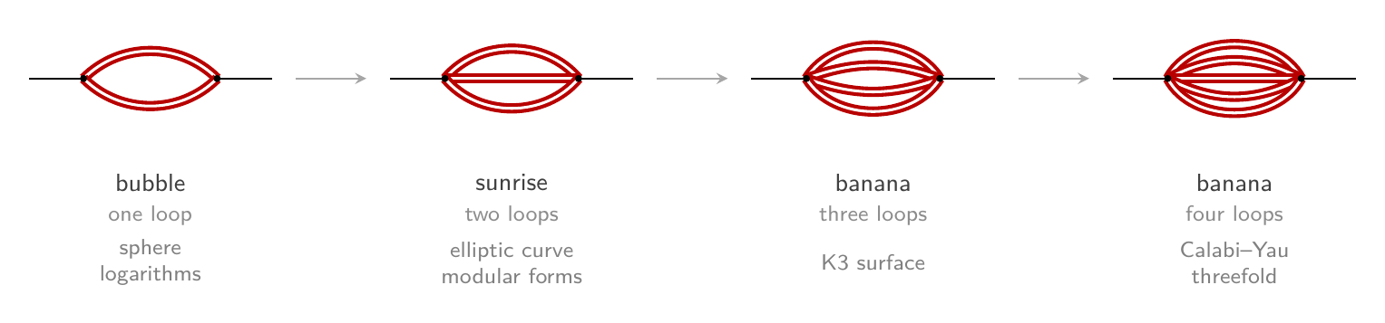
BootLoops was initially designed to solve the integrals associated with Feynman diagrams. Feynman diagrams are a graphical representation of a perturbative expansionsolving a theory as a series of ever-smaller corrections; each order in the series adds diagrams with one more loop graded by loop order:

Every diagram stands for an integral, and they all share one form:
$$I(a_1,\ldots,a_N)\;=\;\int \prod_{\ell=1}^{L}\frac{d^d k_\ell}{i\pi^{d/2}}\;\frac{1}{D_1^{a_1}\,D_2^{a_2}\cdots D_N^{a_N}},\qquad D_j=q_j^2-m_j^2$$
There is one $d$-dimensional integration for each of the $L$ loops, and one propagatorthe factor a virtual particle contributes to a diagram: $1/(q^2-m^2)$ for momentum $q$ and mass $m$ $D_j$ in the denominator for each internal line, where $q_j$ is a fixed combination of the loop momenta $k_\ell$ and the external momenta. A propagator vanishes when its virtual particle goes on shellsatisfies $q^2=m^2$, the energy–momentum relation a real, observable particle obeys — those vanishings are the singularities that make the integrals both hard and interesting. The integrals are computed in $d=4-2\varepsilon$ dimensionsdimensional regularization: working slightly away from four dimensions turns intermediate infinities into poles in $\varepsilon$, which cancel in physical predictions, and the answer comes out order by order in $\varepsilon$: at each order, a function of the external energies and masses. Those functions are what BootLoops computes, and each loop order makes them dramatically harder — multi-scale integrals at two and three loops sit at the frontier of what is computable.
Which functions can appear is set by the geometry of the integrand's singularities. When that geometry is a sphere (genus zerogenus counts a surface's holes — a sphere has genus 0, a doughnut genus 1 — and each extra hole forces harder functions), the answers are generalized polylogarithms (GPLs)nested generalizations of the logarithm — iterated integrals $G(a_1,\ldots,a_n;x)$. Every one-loop diagram is in this class, and the class is thoroughly understood: each integral is built from a finite alphabet of "letters" fixed by its singularities, and is captured by a compact algebraic fingerprint called the symbola Hopf-algebraic shorthand recording which letters appear at which depth of the iterated integral.
One step up the geometry is a torus (genus one), and the functions become elliptic. Massive two-loop integrals live here; the archetype is the equal-mass sunrise — three identical massive lines — expressible in elliptic polylogarithms and iterated integrals of modular formshighly symmetric functions attached to families of elliptic curves — the same objects that starred in the proof of Fermat's Last Theorem. Nothing as simple and universal as the symbol calculus is known here yet.
Beyond the torus sit the K3 surfaces and Calabi–Yau $n$-folds, its higher-dimensional cousins. Their integrals are governed by periodsthe characteristic numbers a geometry yields when integrated over, the way a circle yields 2π — an ellipse's circumference is the first nontrivial example obeying their own (Picard–Fuchs) differential equations, and here no fixed list of special functions suffices: for the cases certified on this site, the space of required functions is provably infinite. From the bubble to the sunrise to the bananas, the geometry and the functions climb together:
Why the difficulty climbs so fast
For the mathematically inclined, the reason is easy to see. These Feynman integrals are all integrals over rational functions — ratios of polynomials. The polynomials in the denominators can vanish so that the integrand becomes singular. The integral can usually still be done. For example, at one loop we may get a logarithm $\int_0^x \frac{dt}{1-t} = -\log(1-x)$. At higher loops we get dilogarithms: $\mathrm{Li}_2(x) = \int_0^x dt \int_0^t ds \frac{1}{t(1-s)}$. At two loops the structure gets richer. After carrying out some of the integrations, the integral may look like $4a \int_0^1 \frac{(1 - e^2 x^2)\, dx}{\sqrt{(1-x^2)(1 - e^2 x^2)}}$. Such an integral is called elliptic. This particular one is exactly the circumference of an ellipse with semi-major axis $a$ and eccentricity $e$. Elliptic integrals cannot be reduced to logarithms or even generalized polylogarithms.
Doing a Feynman integral starts with understanding where the integrand is singular: the singular locus. We handle these singularities by avoiding them: deforming the integration contour into the complex plane, or more generally into ${\mathbb C}^n$. In the complex plane we need Cauchy's theorem and complex analysis; in ${\mathbb C}^n$ we need algebraic geometry.
Much of the exotic geometry needed for Feynman integrals arrived in physicists' vocabulary via string theory. Calabi–Yau manifolds, their periods, and the mirror-symmetry machinery for computing them were developed and made famous by string theory in the 1980s and 1990s. Calabi–Yaus are the extra-dimensional shapes string theorists fold space into, and the celebrated 1991 calculation of the periods of the "quintic" set off the mirror-symmetry revolution. That apparatus turns out to be the natural language for a three-loop diagram you could sketch on a napkin.
The method
The BootLoops approach tries to bootstrap the integrals, using the singularity structure in particular, to figure out much of the answer before even attempting the integral. In the polylogarithmic case, largely due to the power of the symbol, integrals can often be completely fixed by bootstrapping. In the elliptic case, it's more complicated; bootstrap tools constrain the function class of the answer but rarely fully determine it, and sometimes some amount of direct integration is needed. Indeed, BootLoops can also compute the integrals directly, using whatever modern methods are in its toolbox or internalized by the LLM. But the real strength of BootLoops is in combining direct methods with indirect bootstrapping, numerical evaluation, and semi-analytic functional regression. And the architecture is general. It needs three things from a problem: an integral or sequence with a finite singular locus, a function space pinned by that locus, and exact constraints tying coefficients together. Those three recur across the sciences: lattice Green functionsthe functions encoding how a random walker spreads over a crystal lattice — a classic of solid-state physics since the 1930s and spectral moments, cosmological wavefunctions, string integrals, Bayesian evidence in phylogenetics and statistics, the loop kernels of large-scale structure. Anything in the Euler–GKZ / holonomic world is in scope. For loop integrals, the basic algorithm has five steps; other problem classes run the same steps from different entry points.
The step-by-step method
Step 1 — identify the singularities. Everything starts from where the answer can blow up. The complete Landau singular locusthe complex surface on which the integral can be singular is computed three independent ways — PLD and SOFIA for the principal Landau determinantone polynomial whose vanishing marks every place the integral can become singular — technically the discriminant of the Lee–Pomeransky polynomial $\mathcal G = \mathcal U + \mathcal F$; its irreducible factors are exactly the candidate symbol letters with its GKZ certificatea completeness proof, from the Gelfand–Kapranov–Zelevinsky theory of hypergeometric systems, that no candidate singularity was missed, and the Euler-characteristic-drop criterion (Leviathan) — including the second-type and hierarchy-violating singularities no threshold analysis exposes. The output is the alphabet: the finite list of places, and hence letters, the answer is allowed to know about.
Step 2 — identify the function space. The singularities say where; the geometry says what kind of function. The maximal cutthe integral with every propagator put on shell — it isolates the problem's intrinsic geometry is read off (in Baikov's representation, where it becomes an explicit algebraic surface) and classified (GeoTriage): genus 0, elliptic, K3, or CY$_n$ — which fixes the iterated-integral kernels the answer must be built from. The leading singularitythe overall prefactor the whole answer must carry, read off from the integral's singular core rather than by doing the integral supplies the normalization. Alphabet plus kernels plus prefactor generate the weight-graded ansatz: a trial sum of every allowed function of the right transcendental weight (a log counts weight 1, a dilog 2, and so on), with unknown numerical coefficients (Landau Alphabet, Ansatzer).
Step 3 — refine the function space. Exact physics constraints shrink the ansatz before anything is computed: which singularities may appear first, last, or in adjacent slots (first/last-entry and Steinmann conditions), symmetry (parity and crossing), and self-consistency (integrability). The raw ansatz collapses to a residual of $10^2$–$10^3$ unknown numbers, counted exactly before any numerics runs (FORM for the heavy exact algebra, Seedling’s family preflight for the symmetry group actually present, Ansatzer for the exact residual count).
Step 4 — impose numerical constraints. The surviving unknowns are pinned by certified high-precision values of the actual object. Auxiliary-mass-flowadd a fictitious mass that makes the integral easy, then numerically transport the answer back to the physical point at hundreds of digits evaluation (AMFlow) with Kira/FireFly IBP reductionintegration-by-parts identities that reduce the swarm of related integrals in a problem — often millions — to a small independent basis — the "master integrals" — staged by Seedling, with Winnow and Blade as swap-in reducers, and Numkin when multiple symbolic scales stall the reconstruction — generates $\varepsilon$-graded samples at hundreds of digits, taken in the canonical UT basisthe uniform-transcendentality basis fixed by maximal-cut leading singularities plus an IBP rotation — the basis in which weight-graded fitting is meaningful; sampling the raw reduction basis instead produces unfittable mixtures. On the elliptic, K3, and Calabi–Yau rungs the same step runs on certified period transport (Eichler, Coalescer).
Step 5 — determine the constants. The residual is fit by least squares plus per-coefficient PSLQ over a certified constant ring (Lockpick and its constant library); a measured value-fittability triage finds the sectors the fit provably cannot close and sends them to $\varepsilon$-graded Wayfinder transport from analytically derived boundaries. Either way the acceptance test is the same: the claimed form must reproduce independent oracle values at points never used in any fit, to at least thirty genuine digits, two-precision stable (Gatekeeper).
When the steps are not linear. Campaigns off the collider mainline enter wherever their problem lives. Operator-first problems — the Watson integral, for example — start from step 1's geometry and go directly to exact operator reconstruction (Annihilator, Numkin) with step 5's gates. Evidence integrals — phylogenetics, mixture models — are holonomic in the same sense and are solved in closed form at step 3, with no numerics in the result at all. Value-first problems — string integrals, special-point hunts — run steps 4 and 5 — certified evaluation and PSLQ closure — directly against step 1's geometry. The discipline never changes: independent routes to every number and a gate before any claim.
BootLoops Standard
BootLoops ultimately represents one integral (a Feynman integral) as a sum over other integrals (e.g. GPLs or elliptic functions). So what makes the reduced form better, and how does the LLM know when to stop? The BootLoops Amplitude Standard: solving an integral means 1) identifying the functions and 2) having a standalone evaluator that computes the function to arbitrary precision using this functional information. The heart of the standard is that the function be completely characterized — which curve, which level, which kernels. Every constant must be pinned — with a classical name or a special value within the declared function class when possible, but always, at minimum, as a written convergent integral or series with a standalone arbitrary-precision evaluator. The assembled answer must reproduce independent numerics to at least thirty digits, at points never used in any fit, two-precision stable.
The point of a closed form is understanding, and the understanding lives almost entirely in the functions: what functions appear in the answer, and how to characterize them. A numerical evaluation answers "what is the value here"; the identified analytic form answers "what kind of thing is this" — which curve the integral lives on, which modular level, which kernels — and from that, where the thresholdsthe energies where producing a new set of particles first becomes possible — the amplitude develops kinks and branch points there sit, what the asymptotics do, what deforms as the masses move. Alongside the functions come constants. They usually teach us nothing about the integral, but we need them anyway — to pin the answer down and to evaluate it — and they are the most computationally expensive part of the whole program. Some have names, like $\zeta(3)$. Some are defined by a definite integral that no one has ever given a simpler name to. BootLoops produces both the functions and the constants.
This bar is higher than the Feynman-integral community's. The community norm for presenting an elliptic Feynman integral asks for the function part: an $\varepsilon$-factorized differential equation (Adams–Weinzierl 2018), iterated integrals over a declared alphabet (Remiddi–Tancredi 2017, Adams–Weinzierl 2017, Broedel–Duhr–Dulat–Penante–Tancredi 2018), and a boundary value at a cusp or MUM point with numerical cross-checks (Pögel–Wang–Weinzierl 2022a, 2022b). The norm is looser on the rest: boundary constants are routinely left as eMZVelliptic multiple zeta value: the value of an elliptic iterated integral at the cusp, the elliptic analogue of an ordinary zeta value-like special values or plain $q$-series numerics, and blind numerical validation is not uniformly demanded. Most of the time there is no need to do these remaining integrals or identify the constants. BootLoops holds itself to the higher bar deliberately: an LLM ran this pipeline, so every claim — including the uninteresting constants — had to be checkable by machine, start to finish.
The functions
The functions. A polylogarithm never gets "solved" into anything simpler; it is defined by an iterated integral. The logarithm is the name we give $\int_1^x \frac{dt}{t}$. Nesting once more gives a weight-two GPL,
$$G(a_1,a_2;x) = \int_0^x \frac{dt_1}{t_1-a_1}\int_0^{t_1} \frac{dt_2}{t_2-a_2},$$
and the general $G(a_1,\ldots,a_n;x)$ nests $n$ deep, one letter $a_i$ per integration — the dilogarithm, for instance, is just $\mathrm{Li}_2(x) = -G(0,1;x)$. For most GPLs no simpler closed form exists — and none is needed, because the function is completely characterized by finite data: the alphabet of letters and the weight grading, all encoded in the symbol. Identifying a polylogarithmic answer means producing exactly that data, plus the rational prefactors in front, and the bootstrap does much of this efficiently. Elliptic functions are the same story one rung up the ladder of function spaces: functions defined by integrals over a curve, again usually with no simpler form. The prototype is the complete elliptic integral
$$K(k) = \int_0^1 \frac{dt}{\sqrt{(1-t^2)(1-k^2 t^2)}},$$
the basic period of the elliptic curve $y^2 = (1-t^2)(1-k^2 t^2)$ — the square root of a quartic cannot be traded away for simple poles. The functions appearing in elliptic Feynman integrals — elliptic polylogarithms, iterated integrals of modular forms — nest integrations against the curve's differential $dt/y$ the way GPLs nest $dt/(t-a_i)$. The characterizing data, though, is now geometric and arithmetic: which elliptic curve, its conductoran integer invariant $N$ of the curve; it dictates which Dirichlet $L$-values can appear as boundary constants, its cuspsthe boundary points of a modular curve — its points at infinity — where series expansions and boundary values are anchored, which modular forms exist at each weight. The paradigm case is gg→Zγ. The bootstrap's usual endgame — write down every function that could appear, then fit their unknown coefficients against high-precision numerics — cannot work here even in principle: the answer provably lies outside any finite list of weight-graded functions, so there is no ansatz to fit. Instead the amplitude closes as a cusp-regularized Eichler integralan iterated integral of a modular form down from the cusp at i∞, with the divergent piece subtracted on $\Gamma_0(4)$ with Eisenstein kernel $B_{2,4} = E_2(\tau) - 4E_2(4\tau)$, pinned by exactly this arithmetic: the conductor is 4 and not 3, the cusp data, and a modular space with no cusp forms at any weight $\le 4$. That identification says why Catalan's constant can appear in this amplitude while the sunrise's $L(\chi_{-3},2)$ cannot, which expansions converge where, and how the function continues across thresholds.
What "provably impossible" means
These impossibility results are structural, not reports of failed searches — and they come at two levels of rigor. The cleanest is a certified minimal-order theorem: every function in this subject obeys a linear differential equation of some minimal order, and creative telescoping can find that equation and prove none of lower order exists. For the lattice Green function, any candidate of the long-hunted form — a product of two complete elliptic integrals with an algebraic prefactor — automatically satisfies an order-4 equation, while the integral's minimal equation is certified to have order 5. No function satisfies both, so the closed form does not exist for generic rates: decades of failed searches become a theorem. gg→Zγ uses a different lever: the differential equation injects the quasimodular E₂+Eichler content that the Legendre relation forbids any finite weight-graded, constant-coefficient dictionary of polylogarithms from representing — a linear-independence obstruction rather than a transcendence theorem for the specific constants. So no finite fitting dictionary can close it, and the amplitude is delivered as the named modular integral.
The constants
The constants. The cleanest way to get a constant, when it works, is to derive it: impose a condition the function must satisfy — regularity at a threshold, boundedness at a special point, matching at a cusp — and the constant follows exactly, with a reason attached and no integration performed. For example, the ice-cream cone's homogeneous constants follow from matching at the $\infty$-cusp, and the light-by-light kite's threshold turn-on $A_1=-2\pi$ is a theorem, forced by regularity at threshold. The next best way is to evaluate the integral numerically to hundreds of digits and then try to recognize the number. In this case, recognition needs a declared list of candidates. For a polylogarithmic integral the list is a universal ring graded by transcendental weight$\pi$ and a log count weight 1, $\zeta_2 = \pi^2/6$ weight 2, $\zeta_3$ weight 3, and so on; at each order in perturbation theory only one weight appears, known before the calculation starts: powers of $\pi$ and $\zeta$-values — $\zeta_2 = \pi^2/6$ and $\zeta_3$ at low weight, then $\zeta_4 = \pi^4/90$, $\zeta_2\zeta_3$, and $\zeta_5$ above. The list is short and the same for every diagram, so fitting it (with PSLQ or LLL) is a finite question with a yes-or-no answer; the crossed box's anchor constants close in exactly such a weight-graded classical ring.
An elliptic integral's constants instead live in a ring attached to its own curve, and the generators have to be built before they can be searched: the curve's periods, their products with powers of $\pi$, and the Dirichlet $L$-values the curve's conductor selects. The ring is per-diagram rather than universal, and it has no certified dimension, so a null search means only "not in the ring as built" — every null here comes with positive controls and two-precision stability before it is believed. Classical names reappear only where special arithmetic forces them, as in the lemniscatic $\Gamma(\tfrac14)$ ring that closes the CY₃ banana's connection coefficients. And sometimes the closure is a proof that no classical name exists: the unequal-mass kite's boundary transcendental lives on a non-CMcomplex multiplication — extra arithmetic symmetry some special elliptic curves have; CM periods collapse to classical Γ-function values; non-CM periods have no known such collapse conductor-128 curve with a provably non-modular kernel, and the lattice Green function's certified order-5 differential operator proves that the elliptic-integral closed form sought since Watson's 1939 problem cannot exist for generic rates — the answer lives one level up, on the periods of a K3 surface. A boundary period without a classical name is a discovery.
The elliptic tools, by role
Routing: GeoTriage turns maximal-cut geometry and Picard–Fuchs order (2 elliptic, 3 K3, 4 Calabi–Yau) into a value-fittability verdict; unfittable sectors go to Wayfinder. Identification: GeoTriage names the congruence subgroup, Lockpick's constant library the conductor at each cusp (149 digits on the conductor-4 call), Eichler the periods — branch-certified quadrature against the complete-elliptic/AGM route, remainders under proved Arb bounds. Boundaries: the cusp dictionary, the threshold-vacuum anchor, Nestor's subtracted-dispersion module, the p-adic Frobenius bootstrap (an $L$-value to 48 digits, no integral evaluated). Certification: Counterweight proves impossibility when no rational $\varepsilon$-gauge exists, Gatekeeper certifies on the worst withheld point, Coalescer re-derives the K3 coefficient from scratch. Naming: Lockpick/PSLQ — $\pm$ controls, two-precision stability, never-fit acceptance, and a span-deficiency verdict that refuses to invent closed forms (0 of 457 hexa-box constants).
The standard at each rung
- Polylogarithmic — complete closure: the alphabet, the ansatz, and every constant fixed, with the constants in the universal $\zeta$/$\pi$ ring. Nothing is left as numerics.
- Elliptic — the function pinned as a named modular object — which curve, which conductor, which kernels — with boundary constants derived from analytic conditions where possible, otherwise closed in the curve's own ring, and namelessness proved when no classical name exists (the sunrise, gg→Zγ, the kites, the ice-cream cone).
- K3 — the family and its Picard–Fuchs operator identified, and the solution closed through the Frobenius tower at the MUM point with exact connection and boundary coefficients (the three-loop banana with boundary $7\zeta_3$; the threshold banana with $c_{3/2} = -\sqrt{3}/(36\pi)$, an explicit expansion of a Feynman K3 period around a non-unipotent point, with the fractional-branch connection coefficient closed exactly; the lattice Green function and post-Minkowskian two-body K3s).
- Calabi–Yau — the same standard one dimension up, with classical names claimed only where arithmetic forces them (the CY₃ banana's quarter-integer connection coefficients close in the lemniscatic $\Gamma(\tfrac14)$ ring — so far as we can tell, the first $\Gamma(\tfrac14)$ in the banana ladder).
Using the results
For each integral the answer is the exact function. Every diagram page opens with the function itself and closes with the determination record, and files/<name>/ holds the expression document — the closed form with every kernel, constant, and convention written out. Each folder also includes the claim's certificate: a standalone evaluator, plain Python over mpmath, no AMFlow, Kira, or IBP at runtime. Run bare, it rebuilds the result from the exact data included with it and re-measures the acceptance gates against byte-traced oracle values recorded in its header, reserved from every fit. Given a kinematic point, it evaluates the closed form there at any requested precision — and when no recorded oracle value exists at that point, it prints the value and says so, with no agreement claim:
python3 files/sunrise/sunrise-evaluate.py
    # no arguments: recompute the result and check it against the
    # independent reference values included with it

python3 files/sunrise/sunrise-evaluate.py --point=-3.5 --dps 40
    # evaluate the sunrise integral at the momentum p²/m² = −3.5,
    # to 40 digits
Bayesian evidence integrals
The first use case beyond physics was Bayesian evidence. The evidence integral — the probability of the data under a model, averaged over the model's parameters — is, written in Lee–Pomeransky form, the same mathematical object as a Feynman integral: polynomials raised to parametric powers. Phylogenetics, mixture models, population genetics, neutral ecology, and single-cell kinetics all run on it, and for thirty years those fields have estimated it by Monte Carlo. The harness computes it exactly where the model allows and with certified error where it does not: Annihilator turns an evidence integral into an exact recurrence and walks it from a trivial seed; JaCK & Jill returns tree evidence exactly — a ratio of explicit integers — for Jukes–Cantor-class models, and certified enclosures beyond them; Mixalot does mixtures, entity resolution, and authorship; Popcorn runs certified population-genetics likelihoods at biobank scale.
What counts as an answer here. Exactness changes what a result even is. When the evidence is an exact rational number, equality is exact: the two hominid quartet topologies that come out tied are exactly tied, a fact no amount of sampling could establish and no choice of prior or amount of compute could break. An exact result is still gated — it must reproduce an independent high-precision quadrature that was never used in the derivation, the way the first exact phylogenetic Bayes factorthe ratio of two models' evidence — the Bayesian measure of how strongly the data favors one model over the other was checked to 61 digits. Where exactness runs out, the answer is a certified enclosure — an interval proven to contain the truth — never a bare floating-point estimate. Any fast estimator used at scale is calibrated against the exact values it approximates, and the calibration is part of the answer. Every pipeline passes the planted-truth protocol above before it touches real data. And the claim carries its scope printed on it — which models, which sizes, what was not computed — with negative verdicts reported as plainly as positive ones.
Example applications: exact evidence for small phylogenetic trees — the marginal likelihood of a four- or five-species tree computed as an exact fraction, the great apes included; mixture models from two components to infinity; the Federalist Papers, the Shakespeare canon, and the book of Isaiah; whether chance alone explains the species diversity of Panamanian rainforests; and how genes fire in bursts.
Certified arithmetic and audits
A second use case turns the tools on published numbers: star ratings, regulatory thresholds, court-ready estimates, reference tables. The tools are Baller and Arb for computation that carries its own error proof, exact rational arithmetic for replaying published calculations, and Gatekeeper for the provenance of every reference value.
What counts as an answer here. The standard is fail-closed: a result is a certified digit string or a refusal — Baller's solver raises precision until the requested digits are proven, and declines rather than degrade its guarantee. An audited published number lands in one of four classes: it reproduces from the record's own inputs; it is determined only under unstated conventions; it is undetermined; or it is uncheckable — and the classification is the result. Where an audit disagrees with the record, the disagreement is located, not just asserted: the criterion, the step, and the size of the discrepancy, each checkable by rerunning the released evaluator.
Example applications: Medicare's star ratings, measured against the optimality criterion their own rulebooks state; the digit-cutting arithmetic that enforces America's ozone limit; and the population-genetics software behind rare-variant medicine, audited against exact answers.
Exhaustive enumeration and proof
Some questions end only when every case has been checked, and some end in a proof that no case can exist. Terrier runs censuses over string-theory flux latticesthe discrete grid of allowed field-strength settings when string theory wraps fields around a compact shape — each lattice point a candidate vacuum with exact lattice arithmetic; the census engines behind the linguistics results enumerate every stress system a human language can use; Annihilator's creative telescoping turns closed-form questions into provable recurrences of certified minimal order.
What counts as an answer here. A census counts only with its completeness certificate: a mass formula or equivalent identity proving the enumeration missed nothing, and, where feasible, a second enumeration built independently of the first. An impossibility claim must arrive as a theorem — the lattice Green function's long-hunted closed form is excluded because its minimal differential operator is certified to have order 5 while any candidate of that form satisfies order 4. And a suite of solvers earns the right to report failure on a real target only after provably cracking planted instances of the same kind — the discipline behind the Voynich verdict.
Example applications: string theory's flux lattices, censused with completeness guaranteed by mass formulas; the stress systems available to human language, enumerated and proved complete; every mechanical reading of the Voynich Manuscript, run against solvers that provably crack planted ciphers; and the closed form hunted since 1939 for lattice Green functions, proved never to have existed.
How the toolkit grows
A new tool gets written when the existing ones come up short. Across the campaigns the growth events repeat in a few kinds:
- A public engine is ported out of a stack an LLM cannot drive well (Mathematica, MatLab, Stata). AMFlow, the reference evaluator behind most of the amplitude cross-checks, and Blade both run here as ports out of Mathematica.
- An engine hits a wall mid-campaign and gets upgraded, and the upgrade is kept as a fork. The patch rides on a full copy of the upstream project, so the original code, license, and attribution stay intact and the fix can be offered back; the repo's
upgrades/directory collects these. The clearest case is the AMFlow fork, whose series solver had to be rebuilt to keep nearly coincident solution families separated at extreme precision — the worked example at the end of this section tells that story. The same event has milder forms: Kira runs stock, but gained a driver layer and an out-of-tree 128-bit rebuild (kira128) using upstream's own build option — an upgrade with no fork at all.
- A method that exists only in a paper becomes code. Eichler implements the Eichler integrals nothing public would compute; Mixalot implements exact mixture-model evidence from the algebraic-statistics literature, reproducing its benchmark values integer for integer — including one table that had taken 16 days of computer algebra when first published.
- Nothing exists at all, so the tool is built from scratch. The very first gap was the constraint engine itself: PLD and SOFIA can find where an integral is singular, but no public tool turns that singular set into the bootstrap's working ansatz — the symbol alphabet, the first- and last-entry conditions, the integrability and Steinmann cuts, and the residual count that says how many numerical samples will pin the answer. The harness wrote that pair — Landau Alphabet and Ansatzer — before it could solve anything at all. ERAS was born the same way on the applications side, in the linguistics campaign, when naive interval arithmetic returned an enclosure 10²² wide on a likelihood whose true sensitivity is a few hundred; the certified cure is now the arithmetic foundation across the applications.
- A tool built for one problem generalizes on its next encounter. Eichler's arc is told above: one function, then the whole curve family, then K3 and Calabi–Yau periods. Annihilator repeated the arc across fields: built to certify the recurrence operators of Feynman-integral series, it now turns Bayesian evidence integrals into exact recurrences in ecology, single-cell biology, and linguistics.
That cycle — progress, wall, new tool, and around again — built the amplitudes core tool by tool in about three weeks, and it has kept running through every application since. The example below follows a single diagram through four rounds of it.
Example: the tool trail of one diagram
A good example is the kite, a three-loop light-by-light diagram with a two-loop self-energy blob on one rung. Solving it took four rounds of tool-building.

The kite. Wavy lines are the four external photons and red double lines the massive electron; the bottom rung carries the two-loop self-energy blob of the text, whose two massless propagators are the thin black lines. Three loops in all, and the diagram the four rounds below had to solve.
First, AMFlow — the reference evaluator, public code the harness had ported — returned zero correct digits at exactly the limit the calculation needed, with no error message. The harness ruled out the usual suspects, memory and linear algebra, before the trail ended at a judgment call deep in the series solver. When the solver expands around a singular point, the solutions come in families, and it must decide whether the exponents of two families differ by an exact integer, a decision that changes the form of the series itself. It made that call with a fixed tolerance, which is safe at ordinary settings. Here the regulatorthe small parameter ε of dimensional regularization that makes loop integrals finite; physical answers are read off as it goes to zero had to be pushed down to $10^{-120}$, the exponents of two distinct families came that close to coinciding, and the tolerance test merged them: the pole carrying the answer was silently discarded. The harness rebuilt the test to scale with the working precision, so the families stay separated no matter how small the regulator. The same run then gave 160 digits, and the upgraded solver ships as the AMFlow fork in the repo's upgrades/.
Second, the blob's weight function had to be evaluated at 1,669 energies, each evaluation expensive. Rather than compute them all, Wayfinder computed one energy to high precision and carried it to the rest along the function's own differential equation, good to 99 digits per point.
Third, the final integral stalled at six digits. The integration rule assumed a smooth integrand, but the weight function has kinks at the energies where new particle-production channels open, and doubling the node count gained roughly one digit. The harness built a dispersion-integral routine, now the dispersion module of Nestor, which splits the range at the kinks and uses a rule insensitive to them; the integral then converged to 99 digits, and every later diagram with a self-energy blob uses it.
Finally, the comparison against the reference stalled at 18 digits; one culprit was the stored reference value, itself only accurate to 18 digits. Gatekeeper's registry now records the precision and provenance of every reference number. Against a fresh reference, the final value agreed with a fully independent computation to 41 digits.
How to use it
The easiest way to use BootLoops is just to say to your LLM "Install BootLoops".
The harness itself — the toolkit, the ports and engine upgrades, and the protocol skills — lives in a public GitHub repository. To clone it on your local machine just run
git clone <repository-url>      # the link is in the page header
cd bootloops
claude        # Claude Code, or any agentic LLM tool with file and shell access
No GitHub account is needed for this: public repositories clone anonymously. This will clone the full harness: the toolkit, the ports and engine upgrades, and the protocol skills. It's just code, so not terribly large.
By design, the protocol skills arrive inactive; to activate them in Claude Code run /bootloops-setup or just ask Claude to activate the BootLoops protocol skills. The protocol skills can also be installed on their own, without the toolkit, in whichever agent you already use. They follow the Agent Skills open standard, so most agent frameworks read them directly:
- Claude Code —
/plugin marketplace add <plugin-repository>(the BootLoops plugin repository, to be released with the harness), then installbootloops-protocols(the seven working disciplines) and/orbootloops-research(proving with agents, referee audit, literature review, reference checking, prose linting). Updates arrive through the plugin system. - Codex —
codex plugin marketplace add <plugin-repository>: the same two plugins in Codex's plugin format. - Any agent —
npx skills add mattschwartzscience/BootLoopsinstalls skills into whichever agents it finds, with per-skill selection. - Copilot and Cursor — no package needed: both read the skills natively, from a clone or from any of the installs above, and Cursor can import the set straight from the repository link.
- Claude and ChatGPT on the web — the protocol skills run in the web apps themselves: claude.ai takes custom skills as zip uploads in its skills settings, and ChatGPT's workspace plans install them from its plugin directory. For toolkit work the web apps hand off to their cloud coding environments — Claude Code on the web and Codex cloud tasks — which clone the repository into a sandbox with shell access, public repositories included, no fork needed.
On every route the skills are opt-in, and an activated skill only engages when its kind of work comes up.
If all you want is the results from the applications described here, the code for those is stored on bootloops.ai (this site). Simply ask your LLM to pull the code or paper you need from here. It's worth emphasizing that the papers here were almost entirely written by Claude, and they are not written well. To save yourself frustration, a recommended approach is to ask your LLM to read them and to explain to you what is in them. Interrogating the science that way may be more rewarding. On the other hand, the papers are actual self-contained science papers with broad introductions, details, plots, discussion, methodology, etc. So they can be read. Just don't expect Shakespeare (except the quotes in the Shakespeare paper).
Once you have BootLoops installed, to use it, just tell the agent what you want to do. Be as concrete as possible. Name the object if you can: an integral from a paper or a note you give it, or a dataset you want to analyze. The package ships with an LLM-guide: a full toolkit index and detailed guides for all the tools. So ask your LLM first to read the toolkit and catalog which of the tools can help, if any. Although a lot of compute and billions of tokens went into constructing the initial tool library, the tools are cheap to run and a minimal supply of tokens are needed to assess and use them. A laptop and whatever LLM access you already have are enough to drive the code, and you can assess relevance to your problem with free models.