Adaptive trial designs (medicine)
The content on this page was written by AI under human supervision.
Before a Phase II drug trial enrolls anyone, its design is judged on two probabilities: how often it would pass along a drug that does not work, and how often it would catch one that does. For adaptive and Bayesian designs those numbers are almost always estimated by simulating the trial a few thousand times. The paper summarized here measures the noise in those estimates across nine published designs, finds about one in three too close to its threshold to call, and, where a design’s published decision rule allows, computes them exactly instead.
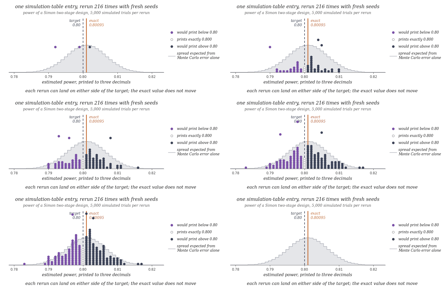
What the simulation noise looks like for a single table entry. Each dot is one rerun, with a fresh random seed, of an entry of the kind examined below: the power of a two-stage design (the Simon design of the first worked recomputation on this page), estimated from 5,000 simulated trials and printed to three decimals as a design paper would print it. Violet dots would print below the design’s 0.80 power target (dashed line), slate dots above it, open dots exactly 0.800; the gray step is the spread that Monte Carlo error alone predicts at 5,000 trials, where one standard error is about 0.006. The exact power, a single fraction computed from the design’s four integers, is 0.80095 (orange line): above the target, although about two reruns in five print a value below it and one in fourteen prints the target itself. (An illustration made for this page from reruns simulated here; not a figure of the paper.)
Judging a trial before it runs
A Phase II trial decides whether a new treatment proceeds to a large confirmatory trial. Its design, the sample sizes, interim looks and rule for declaring the treatment promising, is judged in advance on two probabilities. The type I error ratethe probability that the trial declares an ineffective treatment promising; the design’s false-alarm rate, which a design paper promises to keep under a nominal level such as 5 or 10 percent is the probability that the design carries forward a treatment that does not work. The power is the probability that it carries forward one that does. The pair are the design’s operating characteristics. A design paper states the conclusion they support, that the type I error rate is controlled at ten percent, say, or the power reaches eighty percent, and sponsors and regulators rely on it.
The classic template is the two-stage design Richard Simon published in 1989. Each patient either responds or does not. The design is four integers $(r_1, n_1, r, n)$: enroll $n_1$ patients and stop for futility if $r_1$ or fewer respond; otherwise continue to $n$ patients in all and declare the treatment promising if more than $r$ respond. If the true response rate is $p$, the probability of that declaration is
$$R(p) \;=\; \sum_{x_1 = r_1 + 1}^{n_1} \binom{n_1}{x_1} p^{x_1} (1-p)^{n_1 - x_1} \sum_{x_2 = \max(0,\, r+1-x_1)}^{n - n_1} \binom{n - n_1}{x_2} p^{x_2} (1-p)^{n - n_1 - x_2}.$$Here $x_1$ counts responses among the first $n_1$ patients and $x_2$ those among the rest; each binomial factor is the probability of exactly that many responses, and the limits of the sums encode the two rules. The type I error rate is $R(p_0)$ and the power $R(p_1)$, with $p_0$ the response rate of a useless drug and $p_1 \gt p_0$ that of a useful one. Both are finite sums, exact fractions whenever $p$ is, and optimal designs of this kind are found by evaluating them exactly.
Later adaptive designs add more interim looks and more elaborate stopping rules. Bayesian designs act on posterior probabilitiesthe probability, computed by Bayes’ rule from a prior and the responses seen so far, that the drug’s true response rate lies below (or above) some value; the quantity a Bayesian stopping rule compares with a cutoff; the design BOP2 of Zhou, Lee and Yuan (2017), for example, stops for futility when the posterior probability that the treatment is ineffective exceeds a cutoff that depends on the enrollment so far. Basket designsone therapy tested in several patient subgroups (“baskets”) at once, with a hierarchical model that lets the subgroups borrow evidence from one another through a shared prior on their response rates test one therapy in several subgroups at once and let them borrow evidence through a shared prior. Cutoffs in such designs are usually calibrated, tuned until the type I error rate lies as close under the nominal level as possible.
Simulation tables and their Monte Carlo error
For these designs the standard evidence is a simulation table: the authors run the coded trial a few thousand times under a scenario in which the drug does nothing and again under scenarios in which it works, and report the fraction of runs that declared the treatment promising. Simulation became the standard because the number of ways a multi-arm, multi-look trial can come out grows exponentially while the cost of one simulated trial does not. Each entry is then a Monte Carlo estimate whose uncertainty is fixed by two printed numbers, the estimate $\hat p$ and the number of simulated trials $n$. Its standard error, as Morris, White and Crowther (2019) give it, and the number of runs that would place it two standard errors from a threshold $b$, are
$$\mathrm{MCSE} \;=\; \sqrt{\hat p\,(1-\hat p)/n}\,, \qquad\qquad n \;\gtrsim\; \frac{4\,\hat p\,(1-\hat p)}{(\hat p - b)^2}\,.$$A type I error rate reported as 0.100 from 1,000 simulated trials has a Monte Carlo standard error (MCSE) of about 0.0095. At two standard errors it is compatible with a true rate 1.9 percentage points above or below a 10 percent threshold, so a rerun with a different random seed could land on the other side. The required $n$ grows as the inverse square of the margin, so halving the distance to the threshold quadruples it, and both formulas can be evaluated from a published table alone.
Regulatory guidance already discusses the precision of simulated operating characteristics. The FDA’s 2019 guidance on adaptive designs illustrates precision with 100,000 simulated trials per scenario and allows fewer when the estimate’s whole confidence interval lies below the desired level; the draft international guideline ICH E20 gives the same 100,000 as an example, and both ask that the count be reported with a justification. The paper reads the 100,000 as an example within a requirement of sufficient precision, not as a mandate.
Exact computation instead of simulation
The paper’s starting point is an old fact: for a large class of these designs the simulation was never necessary. Any design whose decision rule depends only on a finite path of integer counts, so many responses among so many patients at each look in each arm, has operating characteristics of the same form as Simon’s:
$$\mathrm{OC}(p) \;=\; \sum_{\text{outcome paths } x} \Pr_p[\,x\,]\; \mathbf{1}\bigl[\text{the event the characteristic counts occurs on } x\bigr].$$The sum runs over every sequence of outcomes the trial can produce; $\Pr_p[x]$ is the probability of that sequence at true response rate $p$, a product of binomial factors and hence an exact fraction; and the indicator $\mathbf{1}[\cdot]$ is one when the design’s rule ends that sequence in the event being counted, a declaration that the drug works. A Bayesian design changes only the condition inside the indicator. In BOP2, with a Beta prior, the posterior probability of futility falls as responses accumulate, so the stopping rule reduces to a table of integer boundaries and the sum is again binomial. Two conditions must hold in practice: the number of terms must be small enough to evaluate, and everything inside the indicator, boundaries, cutoffs, priors and calibration constants, must be stated in full in the paper or its code. In the nine papers examined the second condition often fails, as the recomputation below shows.
To evaluate these sums the author uses the methods of exact multi-loop Feynman-integral computation in physics: dynamic programming with exact rational weights, and quadrature cross-checked by a second schemequadrature is numerical integration, a weighted sum of the integrand at chosen points; here the posterior integrals were computed by one quadrature scheme and checked by an independent one, the two agreeing near the cutoffs to a few parts in a million. For a binary-endpoint design the sum becomes a direct enumeration, or a recursion over the interim looks in exact fractions. For the hierarchical basket designs each term also needs a posterior-tail integral, which in CBHM and BaCIS reduces to nested one- and two-dimensional integrals. These integrals are computed by the cross-checked quadrature. Any outcome whose posterior tail comes out within $10^{-4}$ of its cutoff is left undecided and its probability is added to the width of an interval around the result; an entry is placed above or below its threshold only when that whole interval lies on one side. Each evaluator was checked against an independent exact calculation and, where the design’s authors released code, against that code. Survival-endpoint designs have no finite outcome space; where no exact method exists, the author instead reruns the design authors’ released code, when feasible, at the number of simulated trials the entry’s margin requires, up to two million.
Nine papers and 1,076 table entries
To be examined, a paper had to propose an adaptive or Bayesian design, release its code, and print simulated type I error rates or powers beside a threshold it states, at a stated number of simulated trials. Nine designs contribute table entries: BOP2, BLAST, BaCIS, CBHM, adaptr, ASSISTant, BayesCTDesign, Local-MEM and ScuRMST, published 2014–2026. The paper stresses that these are the whole eligible set rather than a sample, selected for checkability, and infers nothing about papers that publish less.
The nine papers contain 1,076 table entries with a paper-stated threshold. For each, the author computes the margin $|\hat p-b|$ in units of the entry’s own standard error, in exact arithmetic on the printed digits. An entry is undetermined at its reported $n$ when that margin is two standard errors or less, in effect the FDA’s interval condition applied at each paper’s own count. The 281 calibration entries, stated by their papers to be calibrated to the threshold or forced to it by released selection code, are marked; all 150 of ScuRMST’s are among them.
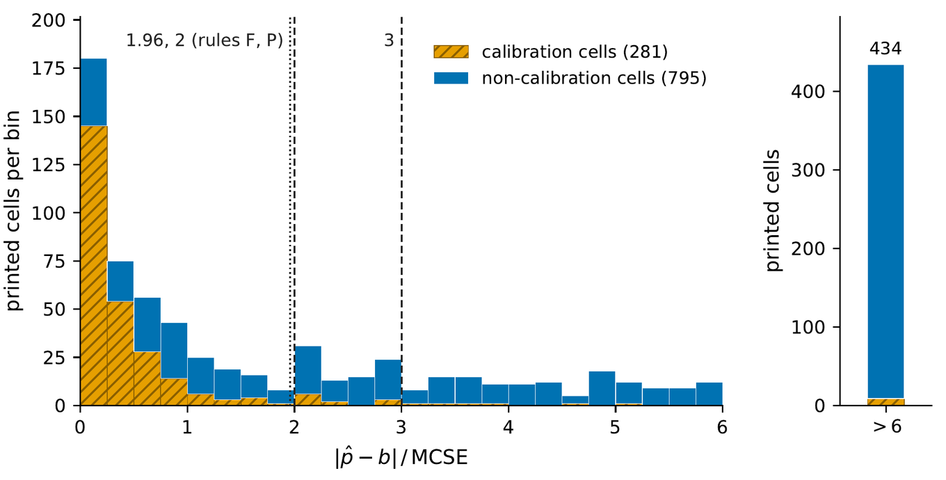
How far each of the 1,076 reported values lies from the threshold it is claimed to clear, in units of its own Monte Carlo standard error at the reported number of simulated trials (the paper’s figure labels the entries “cells”). Hatched orange: the 281 calibration entries, tuned to lie near their threshold and piled below one standard error by construction. Blue: the other 795. The dotted and dashed lines at 1.96 and 2 mark the FDA 95 percent interval and the paper’s primary rule, which classify every entry identically, and a second dashed line marks 3; the right panel collects the 434 entries more than six standard errors clear. In all, 422 entries (39 percent) lie at or below two standard errors and 505 (46 percent) at or below three, and 167 of the 795 non-calibration entries are still at or below two. (Figure 1 of the paper.)
With the calibration entries set aside, 167 of the other 795 (21 percent) still lie within two standard errors of their threshold. Of the 977 entries of the eight designs classified in full (BLAST’s 99, extracted earlier in a feasibility study, get only the margin comparison), 351 are undetermined at their reported count, about one reported claim in three.
The second displayed formula then gives the number of simulated trials each close entry would have needed: a median of 45,697 over the 345 with a nonzero margin, against reported counts of 100 to 10,000. Entry by entry the ratio of required to reported has median 17.7, and for 103 entries the requirement exceeds 100,000. The extreme case is a ScuRMST type I error rate printed as 0.0498 against 0.05 from 5,000 trials, which would take 4,731,997. A further 77 entries are printed exactly at their threshold, and for them the formula gives no finite count at all: a rerun can again land too close to call, and only an exact value determines outright on which side of the threshold the true value lies. One scenario in the nine papers, adaptr’s null, was simulated at the 100,000 of the guidance example.
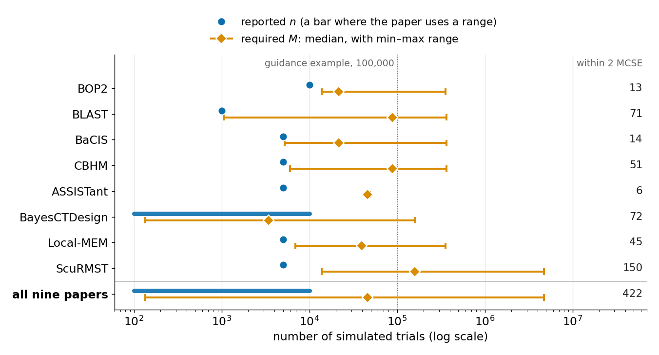
Reported versus required numbers of simulated trials, drawn from the printed values of the paper’s Table 4 (a chart of that table made for this page, not a figure of the paper). Blue: the number of simulated trials $n$ each design paper reports per entry (a bar where the paper used a range). Orange: for the entries of that design lying within two Monte Carlo standard errors of their threshold (count at right), the smallest number $M$ at which the reported value would clear that window, by the second displayed formula; the diamond is the median and the line spans the minimum and maximum, both over the entries with a nonzero margin. adaptr, with no entry inside the window, has no row, and the pooled bar of reported counts, 100 to 10,000, covers the eight designs shown, not adaptr’s null scenario at 100,000. For each design reported at a single count the required median lies to its right; entry by entry the ratio of required to reported has median 17.7 with quartiles 4.3 and 71.4, and the largest requirement, 4,731,997 for a ScuRMST entry printed as 0.0498 against 0.05, lies far beyond the 100,000 of the regulatory guidance’s worked example (dotted line). (Data of Table 4 of the paper.)
Recomputing the close calls
Counted by design class, 597 of the 977 entries (61 percent) are finite sums or low-dimensional integrals of the kind above, whether or not the rule needed to evaluate them is published. The author set out to recompute each of the 351 undetermined entries, exactly wherever the published decision rule was complete and otherwise by re-simulation.
For 152 of the 351 the published materials were enough to begin a recomputation, and 126 were decided: in 87 the recomputed value confirms the reported side; in 30, the reversals, it falls on the other side; and 9 were entries printed exactly at their threshold, which only the recomputation could place. Sixty-seven of the 126 decisions are exact, and eleven entries stayed within two standard errors at the largest counts run and were left without a side. In every reversal the recomputed value lies within 2.2 standard errors of the printed one, so none is an error by the paper concerned. The paper states explicitly that no design, table or approval is called wrong anywhere in it. Under an illustrative binomial model written down before any entry was recomputed, reversals came about as often as Monte Carlo noise alone predicts.
For 211 of the 351, three in five, no recomputation is possible by any method, because a specific input is missing from the published materials. ScuRMST accounts for 150, because its critical values were not archived; the other 61 are entries for comparators (existing designs a paper tabulates beside its own), sensitivity analyses or appendix designs in CBHM, Local-MEM, BOP2 and BaCIS whose analysis rules, cutoffs or parameters appear neither in the papers nor in their released code. A later release of any missing input would make its entries computable under the same rules.
The paper gives three recomputations in full; the simplest concerns a Simon two-stage design used as a comparator in Local-MEM’s Table 3. Its power, by the first equation on this page, is a single fraction, 0.800947…, above 0.80 by construction because the design was selected to have power at least 0.80. The Local-MEM paper reports it in ten entries as 0.792 to 0.806 from 5,000 simulated trials, where the standard error is about 0.006. The five below 0.80 are ordinary Monte Carlo draws of a quantity whose exact value is 0.80095, and each is a reversal.
The second of the three full recomputations concerns the calibration scenario of the basket design CBHM, whose code is distributed with calibrated cutoffs. The calibration row of its Table 1 reports type I error rates of 0.099, 0.098, 0.098 and 0.100 in four subgroups from 5,000 trials, against a 10 percent target. The recursion at the distributed cutoffs, each posterior tail computed by the cross-checked quadrature, places the exact rates in [0.103073, 0.105752] for subgroups 1 and 3, [0.108407, 0.108718] for subgroup 4 and [0.086851, 0.096344] for subgroup 2: above the target in three of four. The printed values are consistent with Monte Carlo error at 5,000 trials, each within about two standard errors of the exact values; the CBHM paper’s own cutoffs are not archived, so the computed intervals describe the design as distributed. Run at its own chain length of 30,000 sampler draws, the released code reproduces the printed value: 0.098 in subgroup 1, against 0.099 printed and 0.104 exact. The gap between the printed row and the exact intervals is thus of the size that a chain of that length produces, not one that more simulated trials would remove.
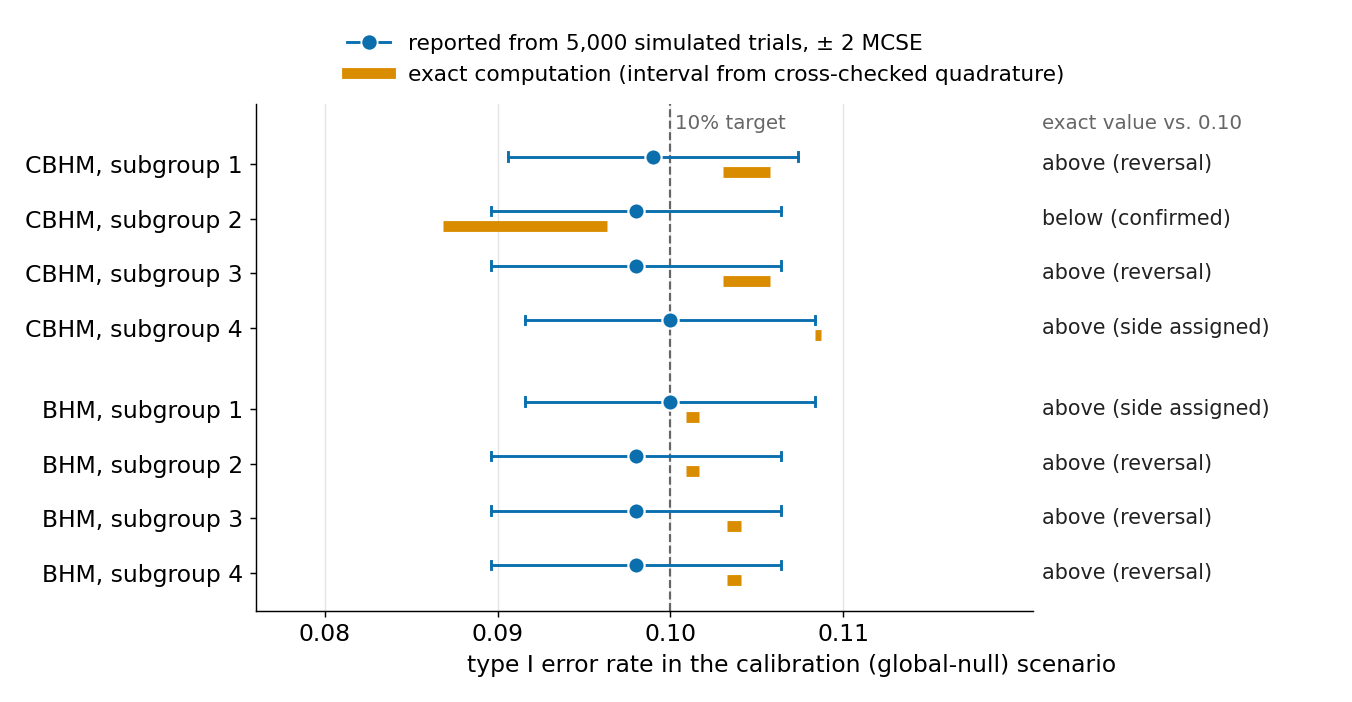
Exact versus simulated for the table row the paper works through in most detail: the calibration scenario of the basket design CBHM and, below, its BHM comparator (the plain Bayesian hierarchical model the CBHM paper tabulates beside its own design), drawn from the printed values of the paper’s Table 6 (a chart of that table made for this page, not a figure of the paper). Blue dots: the type I error rates the CBHM paper reports from 5,000 simulated trials, with bars of two Monte Carlo standard errors (one standard error is about 0.0042 near 0.10, as that table’s caption gives). Orange segments: the intervals in which the exact computation, the recursion with cross-checked quadrature, places the type I error rate at the cutoffs distributed with the design’s code; subgroups sharing a cutoff share an interval. Every reported value lies within about two standard errors of its interval, so nothing in the CBHM table is in error, yet the exact rate lies above 0.10 in three of four CBHM subgroups and in all four BHM subgroups; the two entries printed as exactly 0.100 can be placed only by the exact computation. (Data of Table 6 of the paper.)
Of the thirty reversals, ten arise from calibration to a constraint, as in the Simon case. Two arise from test discreteness, treated in the third full recomputation: the actual type I error rate of BayesCTDesign’s test oscillates around its nominal 0.05 as the sample size changes, between 0.0488 and 0.0516 over the binomial-endpoint entries computed exactly. The other eighteen are plain Monte Carlo side errors. In twenty of the thirty the recomputation evaluates the design paper’s own rule and cutoffs; the other ten (five at the cutoffs distributed with CBHM’s code, five at cutoffs re-derived from its calibration rule) compare the printed estimate with the design as released or as recalibrated rather than with the paper’s own instance. An appendix describes the eleven entries that re-simulation left undecided, among them a Weibull power entry printed as 0.798 that came out at 0.800021 after two million trials.
Reporting suggestions and limits
For the design classes examined, the paper suggests in its discussion four reporting items, two of them already in the guidance. First, the number of simulated trials can be chosen in advance, by the second formula above, from the smallest margin the authors need to resolve, and reported with that calculation. Second, the Monte Carlo standard error can be printed beside every simulated operating characteristic, so that a reviewer can compare an estimate’s distance from its threshold with twice that number. Third, the decision rule can be published in full, with calibrated cutoffs, critical values, comparator rules and the random seed; where papers did so, their tables could be regenerated from the released code. Fourth, where the operating characteristic is a finite sum or a low-dimensional posterior integral, its exact value can be reported instead of an estimate, for the cost of the arithmetic alone.
The paper is explicit about its limits: the corpus is small, and the four designs too costly to re-simulate had no reference reruns; their close entries were settled only where an exact evaluator existed. To the author’s knowledge the classification, which the paper calls its census, is the first measurement of published design tables against the guidance’s precision conventions, and no other priority is claimed. The sibling pages on Medicare star ratings and the ozone air-quality standard follow the same approach: compute exactly a quantity that is approximated in practice, and compare the published numbers with the exact value.
The paper
- Exact versus simulated operating characteristics of published adaptive and Bayesian trial designs (PDF) — Matthew D. Schwartz; a draft dated September 2026. In it the author measures the Monte Carlo precision of the 1,076 simulated type I error rates and powers that nine published adaptive and Bayesian design papers report beside a stated threshold, recomputes the undetermined entries, exactly or by re-simulation, wherever the published materials allow, and suggests four reporting items.
Supplementary material
Files hosted on this site. The script reads the archive directly, so the two are meant to sit in the same folder.
- trials-census.zip — the per-design cell files for all 1,076 entries, with the dated protocol documents, the nine verification records and the analysis scripts, among them the one that draws Figure 1 of the paper; a manifest inside lists every file with its sha256.
- trials-evaluate.py — Python, standard library only. Reads the cell files straight from the archive, checks each against the manifest, and recomputes in exact arithmetic the tallies quoted on this page: 351 of 977, the 77 threshold-valued entries, the median of 45,697. It also computes from scratch the Simon comparator’s power of 0.80095 and the roughly 4.7 million runs the 0.0498 entry would need, in seconds.
References
| U.S. Food and Drug Administration, Adaptive designs for clinical trials of drugs and biologics: guidance for industry, U.S. Department of Health and Human Services (2019) | the guidance with the 100,000-trial worked example and the confidence-interval condition applied here |
| International Council for Harmonisation of Technical Requirements for Pharmaceuticals for Human Use, ICH E20: adaptive designs for clinical trials, draft guideline (2025) | the draft international guideline giving the same 100,000 example and asking that the count be justified |
| T. P. Morris, I. R. White and M. J. Crowther, Using simulation studies to evaluate statistical methods, Stat. Med. 38 (2019) 2074 | the Monte Carlo standard error of a simulated estimate and the number of repetitions a precision requires |
| E. Koehler, E. Brown and S. J.-P. A. Haneuse, On the assessment of Monte Carlo error in simulation-based statistical analyses, Am. Stat. 63 (2009) 155 | found Monte Carlo error rarely reported in published simulation-based analyses, and often material |
| K. Luijken et al., Replicability of simulation studies for the investigation of statistical methods: the RepliSims project, R. Soc. Open Sci. 11 (2024) 231003 | re-ran published simulation studies in biostatistics to measure how much results change on replication |
| R. Simon, Optimal two-stage designs for phase II clinical trials, Control. Clin. Trials 10 (1989) 1 | the two-stage template whose type I error rate and power are exact binomial sums |
| C. Jennison and B. W. Turnbull, Group Sequential Methods with Applications to Clinical Trials, Chapman & Hall/CRC, Boca Raton (2000) | operating characteristics of group-sequential designs from deterministic recursions, without simulation |
| H. Zhou, J. J. Lee and Y. Yuan, BOP2: Bayesian optimal design for phase II clinical trials with simple and complex endpoints, Stat. Med. 36 (2017) 3302 | BOP2, whose posterior stopping rule reduces to integer boundaries; one of the nine designs examined |
| Y. Chu and Y. Yuan, BLAST: Bayesian latent subgroup design for basket trials accounting for patient heterogeneity, J. R. Stat. Soc. C 67 (2018) 723 | BLAST, the basket design whose 99 entries, extracted in an earlier feasibility study, get only the margin comparison |
| N. Chen and J. J. Lee, Bayesian hierarchical classification and information sharing for clinical trials with subgroups and binary outcomes, Biom. J. 61 (2019) 1219 | BaCIS, the hierarchical basket design whose posterior tails reduce to nested one- and two-dimensional integrals |
| Y. Chu and Y. Yuan, A Bayesian basket trial design using a calibrated Bayesian hierarchical model, Clin. Trials 15 (2018) 149 | CBHM, the basket design whose calibration row is recomputed exactly above |
| Y. Liu, M. Kane, D. Esserman, O. Blaha, D. Zelterman and W. Wei, Bayesian local exchangeability design for phase II basket trials, Stat. Med. 41 (2022) 4367 | Local-MEM, whose Simon comparator has the exact power 0.80095 behind five reversals |
| B. S. Eggleston, J. G. Ibrahim, B. McNeil and D. Catellier, BayesCTDesign: an R package for Bayesian trial design using historical control data, J. Stat. Softw. 100(21) (2021) 1 | BayesCTDesign, whose test’s actual type I error rate oscillates around 0.05 with the sample size |
| J. He, R. Lin, Y. Chen and K. F. Lam, Two-stage double-arm trial optimal design of restricted mean survival time with sculpted critical region, Stat. Med. 45 (2026) e70589 | ScuRMST, whose 150 calibration entries cannot be recomputed because its critical values were not archived |
| T. L. Lai, P. W. Lavori and O. Y.-W. Liao, Adaptive choice of patient subgroup for comparing two treatments, Contemp. Clin. Trials 39 (2014) 191 | ASSISTant, adaptive subgroup choice with rank statistics; one of the nine designs examined |
| A. Granholm, A. K. G. Jensen, T. Lange, A. Perner, M. H. Møller and B. S. Kaas-Hansen, Designing and evaluating Bayesian advanced adaptive randomised clinical trials: a practical guide, Pharm. Stat. 24 (2025) e70042 | adaptr, whose null scenario was simulated at the 100,000 trials of the guidance example |