Single-cell RNA bursting (genomics)
The content on this page was written by AI under human supervision.
Genes make RNA in bursts, and each gene is summarized by how often it fires and how much it makes each time, two numbers inferred from RNA counts in hundreds or thousands of single cells. The two papers behind this page compute the probability of those counts exactly. The first rechecks a genome-wide set of published fits and works out how many cells a snapshot would need before it could show that a promoter takes recovery time between bursts. The second uses time-resolved counts to find mouse genes whose promoters wait days between bursts and return through several steps.
Two kinds of time in mammalian promoters — a six-minute telling of the second paper on this page: most classifiable mouse genes switch on at random, but one in seven of them waits days between bursts on a regular clock whose length tracks the methylation of its promoter — the matrix and secreted-protein genes that build the world outside the cell. (Download the video, 14 MB.)
Genes fire in bursts
A gene is not transcribed at a steady trickle. Its promoter, the stretch of DNA where transcription starts, switches on, polymerases run off a batch of transcripts, and it switches off again. Bursting was filmed in single bacteria in 2005 and in a slime mold in 2006, and found in mammalian cells the same year by counting RNA molecules cell by cell.
The standard description is the telegraph model of Ko (1991) and Peccoud and Ycart (1995). A promoter flips from OFF to ON at rate $k_{\rm on}$ and back at rate $k_{\rm off}$, makes transcripts at rate $k_{\rm syn}$ while ON, and each transcript decays at a rate that sets the unit of time. Two combinations summarize a gene: the burst frequency $k_{\rm on}$ and the burst size $k_{\rm syn}/k_{\rm off}$, the number of transcripts a typical burst produces. A cell can turn a gene up either way, so whether a given piece of regulatory DNA acts on frequency or on size is a question about mechanism.
Deciding between frequency and size for every gene in the genome means inferring the rates from single-cell RNA sequencing, which counts each gene’s transcripts cell by cell; in hybrid mice from two inbred strains the two copies of every gene are counted separately. Larsson and colleagues did this in 2019 and fitted the telegraph model to every gene with a program called txburst. They reported that burst frequency is encoded mainly in enhancers, regulatory DNA that can lie far from the gene, and burst size in core promoters. The counts are small, zero in most cells, and the whole inference rests on the probability the model assigns to them.
From counts to rates
At steady state the telegraph model predicts a definite distribution for the count $n$ in a cell. The promoter’s recent activity acts as a random dimmer $u$ between zero and one, and given the dimmer setting the count is Poisson:
$$P(n)=\int_0^1 \mathrm{Pois}(n;\,k_{\rm syn}u)\,\mathrm{Beta}(u;\,k_{\rm on},k_{\rm off})\,du .$$Here $\mathrm{Pois}$ is the Poisson probability of $n$ at mean $k_{\rm syn}u$ and $\mathrm{Beta}$ is the Beta density, shaped by the two switching rates so that a rarely-on promoter puts most weight near $u=0$. The integral has a closed form in Kummer’s confluent hypergeometric function ${}_1F_1$. A gene’s log-likelihoodthe probability that the model, at given rates, assigns to the counts actually observed; the fitted rates are the ones that make it largest is the sum of $\log P(n_c)$ over its cells $c$. The fitted rates maximize it, and the error bars come from how fast it falls away from the maximum. txburst computes the integral with a 50-point quadrature rule and adds $10^{-10}$ to each probability before the logarithm, a routine guard against $\log 0$. Neither it nor any other implementation the authors examined reports an error bound on its value.
The first paper evaluates the likelihood exactly. Written as a power series, the closed form alternates in sign and loses its digits to cancellation once $k_{\rm syn}$ is large; Kummer’s transformation turns it into a series with all terms positive, so nothing cancels and the tail past a known index is bounded. Two such sums at the top of the count range then seed a three-term recurrence for every other probability:
$$n(n{+}1)\,P(n{+}1) \;=\; n\,(n+k_{\rm on}+k_{\rm off}+k_{\rm syn}-1)\,P(n)\;-\;k_{\rm syn}\,(n+k_{\rm on}-1)\,P(n{-}1).$$Willmot and Panjer wrote this recurrence down in the actuarial literature in 1987; as far as the authors could determine, no gene-expression tool had used it. The recurrence has to be run downward: run upward from $P(0)$ it amplifies rounding error, and in one tested regime no correct digit was left by $n\approx200$; run downward it loses about one digit in 1,500 steps. The computation is done in ball arithmeticcomputing with intervals instead of numbers: every quantity is stored as a midpoint plus a radius proven to contain the true value, and every operation updates both; a standard tool of computer-assisted proofs, so each likelihood value comes with a proven error bound. A gene’s probability vector takes about 11.7 milliseconds, five to eight times the quadrature’s cost and cheap enough to use everywhere.
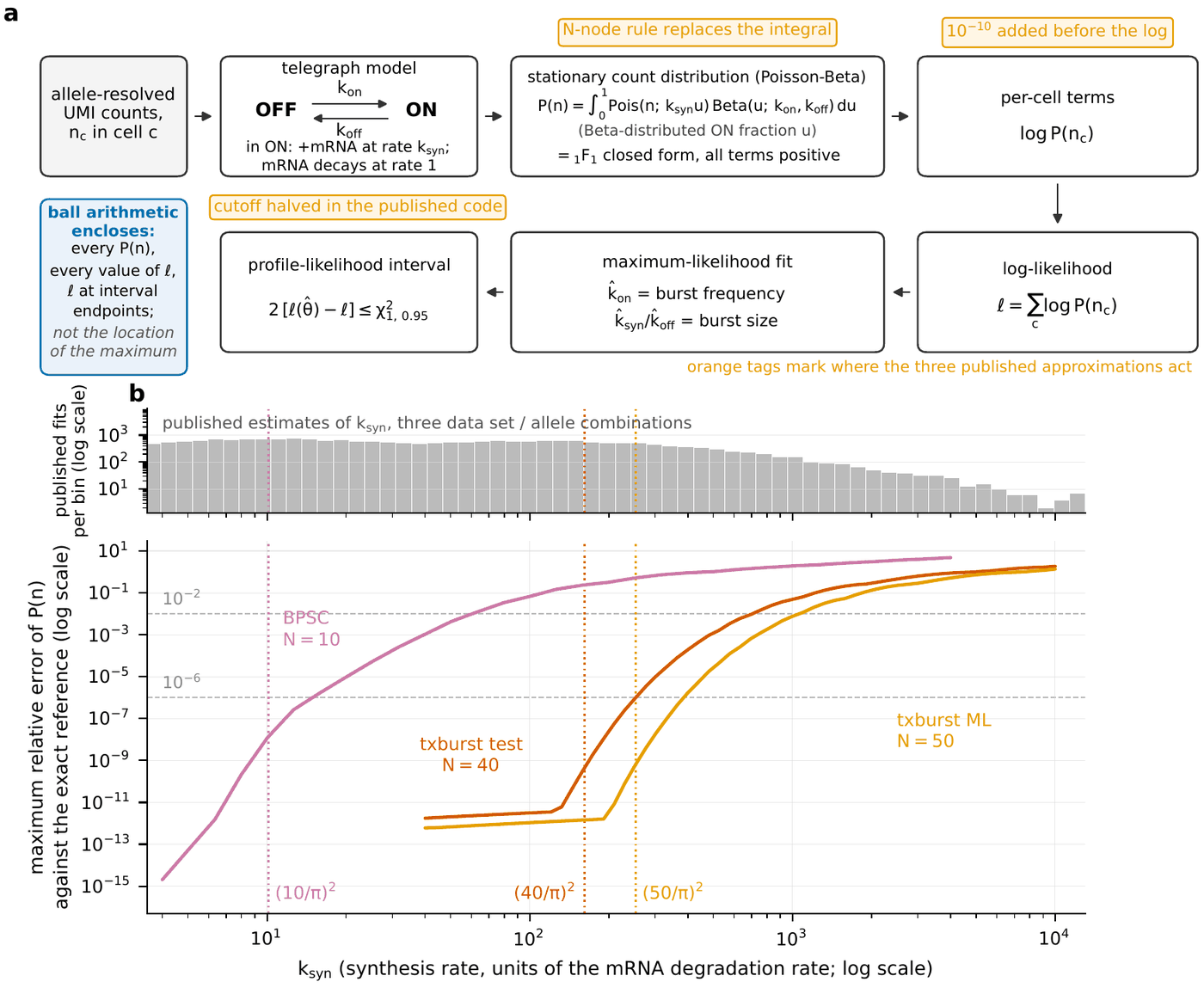
The inference chain and where fixed quadrature gives out. Top, the objects of the problem, from a gene’s counts through the telegraph model and its count distribution to the fitted rates and their error bar; orange tags mark the three places the standard software approximates, and the blue box says what evaluation in ball arithmetic guarantees. Bottom, the largest relative error of an $N$-point quadrature rule against the exact reference as the synthesis rate $k_{\rm syn}$ grows, under a histogram of the 32,376 published estimates: each rule is accurate until roughly $k_{\rm syn}\approx(N/\pi)^2$ and fails beyond it, and most published fits sit below the onset of txburst’s 50-point rule. (Figure 1 of the first paper.)
Rechecking the published fits
Re-evaluating all 32,376 fits of Larsson and colleagues at their own parameters, the authors find that about 99% agree with the exact log-likelihood to better than a thousandth of a natural-log unit. A group of 205 is off by more than one unit, one by 4,827, and few of those lie beyond the quadrature onset. In nearly all of them some cell carries a count that is nearly impossible under the fitted model; the added $10^{-10}$ caps that cell’s penalty, and the program reports a better fit than the model allows. Refitting on the exact likelihood moves burst frequency or size by more than one half-width of even the narrower conditional error bar (the other rates held fixed) for just 12 of 20,201 quality-filtered genes. The published point estimates stand.
The published error bars, unlike the point estimates, need recomputing. An interval ends where the log-likelihood has fallen a prescribed amount below its maximum. One line of txburst’s interval routine halves that amount, applying the cutoff meant for the drop to twice the drop, so nominal 95% intervals are 83.4% intervals. Error bars meant to miss the true value one time in twenty miss it about one time in six. Rescaling is only part of the repair: for 2,066 of the 7,177 genes with reproducible published intervals (28.8%) an endpoint also moves by more than 10% under the exact likelihood, for 309 of them by more than half. Whether any biological conclusion of Larsson et al. changes was not tested.
The authors then take deeper data, 682 fibroblasts of the same cross from one animal, sequenced by Johnsson and colleagues in 2022, and ask a question of their own: which parameter differs when a gene’s two copies burst differently. Of 198 genes tested with exact likelihoods, 104, roughly half, differ between the copies, 77 of them cleanly, with balanced counts and no sign of a mapping or fitting artifact. Separate tests of burst frequency and burst size resolve which parameter for only 19 of the 77, with allelic differences of about twofold: 17 in frequency, 2 in both and none in size alone. That split is a poor guide to how often each mechanism occurs, because the tests have unequal power: at these expression levels a twofold difference in frequency is detected 74% of the time, in size only 36%. In simulations of the whole procedure an even mixture of the two mechanisms gives a split at least this uneven about four times in five, so the authors make no statement about which parameter regulatory differences move more often. Jiang and colleagues (2017) had concluded from the program SCALE that they act overwhelmingly on frequency, and Larsson et al. that enhancers set frequency and core promoters size; the new calls test neither claim.
The limits of snapshot data
In live-cell recordings many promoters are refractory: after a burst they pass through more than one slow step before they can fire again, so their silences are more regular than a single random switch allows. The first paper also evaluates the count distribution of such a two-step promoter exactly.
Exact evaluation controls the numerical error, but the information in snapshot counts sets a harder limit on detecting a refractory promoter. If a gene’s counts come from a two-step promoter, the expected evidence from $n$ cells against the closest telegraph distribution, the average log-likelihood ratio, is $n\,\mathrm{KL}$. Here $n$ counts cells, as in the figure below, and $\mathrm{KL}$ is the Kullback–Leibler divergence between the two distributions, a standard measure of how distinguishable they are. Near-certain detection needs $n\,\mathrm{KL}$ to reach about 8. Across 20,216 genes of the 2019 data, each at its own cell count and fitted rates, the largest value is 0.58, for Timp1 with 224 cells. No gene in that data set was measured in enough cells to reveal whether its promoter needs recovery time between bursts. A gene with the median fibroblast parameters would need at least $1.2\times10^{5}$ cells sequenced as these were, and $3.9\times10^{8}$ if the counts were thinned further to a droplet-like 6% of this experiment’s capture. With every transcript counted the same gene would still need $1.0\times10^{4}$ to $4.3\times10^{4}$ cells, depending on the experiment’s unknown capture efficiency (taken as 10% to 50%). These figures bound only the two-step case; silences with more steps are not bounded.
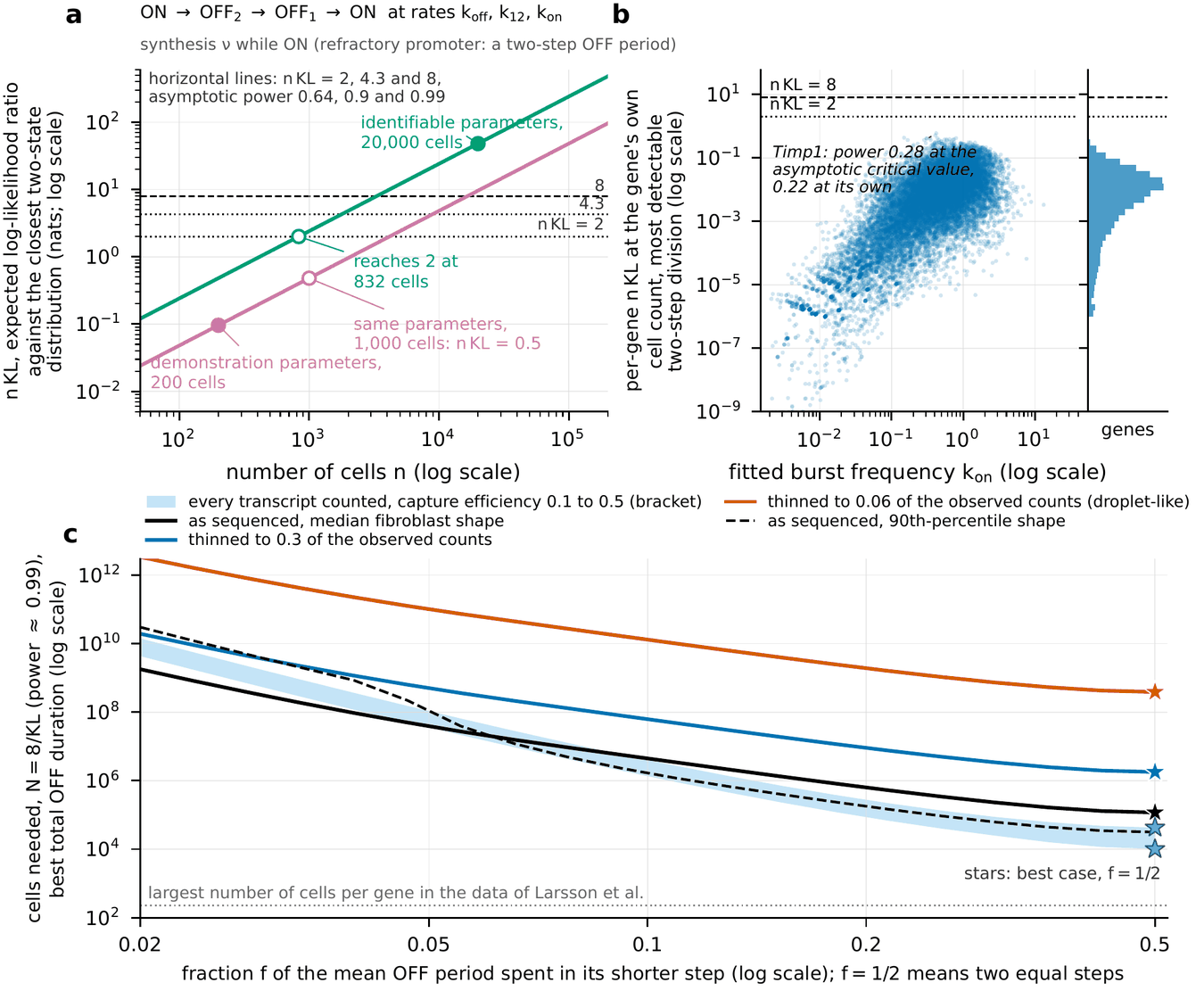
How many cells it takes to see a refractory step in snapshot counts. (a) The expected evidence $n\,\mathrm{KL}$ for a two-step silent period grows in proportion to the number of cells; horizontal lines mark the evidence needed for detection power 0.64, 0.9 and 0.99. (b) That evidence for each of 20,216 genes in the data of Larsson et al. at the gene’s own cell count: every gene falls short of even the weakest line, the best being Timp1 at 0.58. (c) Cells needed for power 0.99 at the median fibroblast parameters, against how the silent period is divided between its two steps: as the cells were actually sequenced (black), and with the observed counts thinned to 0.3 (blue) and to a droplet-like 0.06 (orange) of that. The best cases (stars) are $1.2\times10^{5}$, $1.8\times10^{6}$ and $3.9\times10^{8}$ cells. The shaded band is the same gene with every transcript counted, for an experimental capture efficiency between 0.1 and 0.5, reaching $1.0\times10^{4}$ to $4.3\times10^{4}$ cells at best, still far above the largest cell count per gene in the data (dotted line). The curves bound the two-step case only. (Figure 5 of the first paper.)
Adding a clock to the counts
The second paper uses a different kind of data rather than more cells. In metabolic labeling, cells are fed 4-thiouridinea modified uridine that cells build into new RNA in place of ordinary uridine; a chemical treatment before sequencing makes incorporated labels read as C instead of T for a set time, and RNA made in that window carries a mark that sequencing can read, so every molecule is called old or new. The NASC-seq2 data of Ramsköld and colleagues (2024) give old and new counts of every gene in 8,916 primary mouse fibroblasts after a two-hour window, with the new RNA also resolved by gene copy.
Two hours is comparable to a typical fibroblast promoter’s own timescales: a few hours silent and about two hours active at the median. A snapshot constrains the silent period mainly through its mean; a new-RNA count built up from zero over a known interval also depends on its shape, and the competing models differ only in that shape. In the two-state model the promoter leaves its one silent state at rate $k_{\rm on}$; in the multi-step model it passes through $k$ silent states in sequence, leaving each at rate $k\,k_{\rm on}$. As functions of the waiting time $t$, the silent-period densities are
$$f_1(t)=k_{\rm on}\,e^{-k_{\rm on}t},\qquad f_k(t)=\frac{(k\,k_{\rm on})^{k}\,t^{\,k-1}}{(k-1)!}\,e^{-k\,k_{\rm on}t}.$$Both have mean $1/k_{\rm on}$. The exponential is memoryless: however long a promoter has been silent, its chance of firing in the next minute is unchanged. The second, an Erlang density, is the waiting time for $k$ random steps in a row. Its variance is $k$ times smaller and it has almost no weight near zero, so a promoter that has just fired is unlikely to fire again at once, which is what refractory means. Everything else is shared, including the mean count.
For each gene and trial set of rates, promoter state plus old and new counts form a finite Markov chain, started at stationarity when the label goes on and propagated across the window by uniformizationa classical way to compute how a continuous-time random process evolves over a fixed time, as a sum of non-negative terms whose omitted remainder is known exactly. The uniformization series is truncated once the neglected probability is below $10^{-13}$, so every computed distribution carries an explicit error bound and no simulation noise. Convolution over the two gene copies, a one-in-ten chance that a new molecule reads as old, and random thinning of the molecules to each cell’s sequencing depth then give the probability of what was observed. The two models have the same three free rates and neither contains the other, so the $P$ value cannot be read off a textbook chi-square curve; the authors compute it exactly for each gene under that gene’s fitted two-state model.
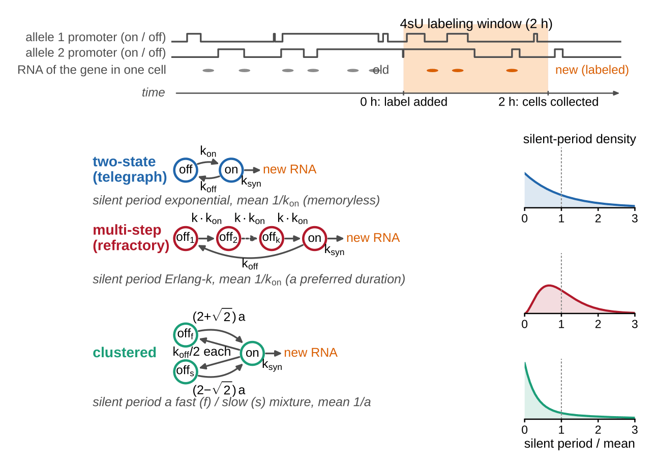
The labeling design and the three promoter models. Top: during a two-hour 4-thiouridine window each new transcript is marked, so a cell reports old and new molecules of every gene, drawn here for a gene’s two copies. Below: the two-state, multi-step and clustered promoters, identical except in how they return from silence, and at right their silent-period densities at equal mean: memoryless, peaked at a preferred duration, and a fast/slow mixture. Only the shape of the silence separates the models, and a new-RNA count built up over a known window is sensitive to that shape where a snapshot is not. (Model diagrams as in Figure 1A of the second paper.)
The refractory class
The two-state and two-step fits both converged for 16,858 of 23,246 genes, and the exact test rejects the telegraph model for 3,737 of them at a 5% false-discovery rate. Three controls then guard against two effects the model leaves out, cell-to-cell variation in capture and the doubled gene copies of cells that have replicated their DNA. Genes whose statistic clears a fixed threshold, is at least three times what gene-matched two-state simulations of either effect produce, and stays multi-step in unreplicated cells alone form the refractory class: 186 genes. Another 1,060 clearly favor the two-state model; 329 of those fit better still with a “clustered” silence that mixes a fast and a slow timescale, less regular than memoryless rather than more. The refractory class is thus 15% of the 1,246 classifiable genes and 1.1% of those evaluated; the other 15,612 are undetermined at this depth, where a two-step silence shows only for genes with long silences and large bursts. Two steps is only a lower bound: for 168 of 184 refractory genes profiled the likelihood still rises at twenty steps, the most regular shape tried.
Among the class’s 164 genes with functional (Gene Ontology) annotations, cell-cycle genes set aside, 62 encode proteins of the extracellular region, a 4.8-fold enrichment, and extracellular-matrix genes are enriched 7.9-fold: genes for what a fibroblast secretes and builds outside itself. The median silent period is 95 hours against 3.9 for two-state genes, and 171 of the 186 have mean silences longer than a 20-hour cell cycle. With active periods three times longer and bursts twice as large, a refractory gene is transcribed for a few hours roughly every four days.
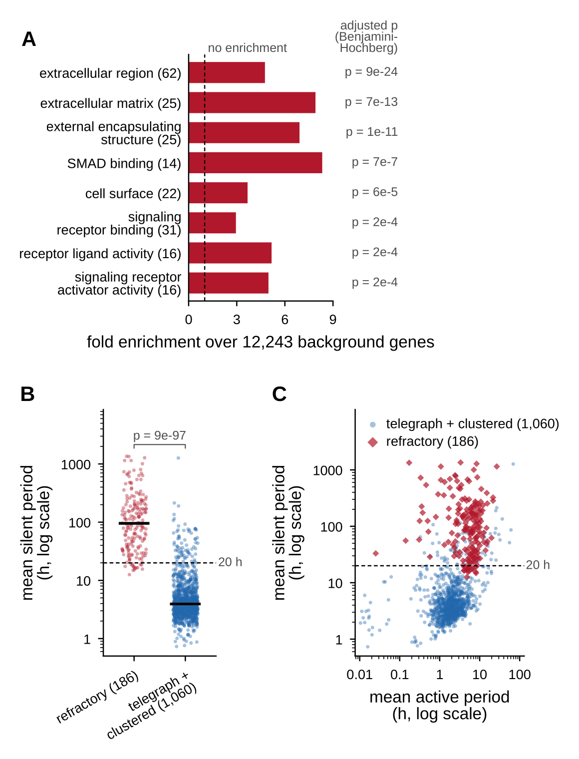
Which genes are refractory and how long they stay silent. (A) Gene Ontology terms enriched among refractory genes against the 12,243 annotated evaluable genes, with adjusted $p$ values at right: secreted and matrix proteins are the most significant, at 4.8- and 7.9-fold. (B) Mean silent period per gene, refractory against two-state: medians of 95 and 3.9 hours, with 171 of the 186 refractory genes silent for longer than a 20-hour fibroblast cell cycle (dashed line). (C) Silent period against active period per gene: refractory genes combine long silences with long active periods; at this depth a multi-step silence can only be detected for genes with long silent periods and large bursts, so part of the separation is selection. (Panels A–C of Figure 2 of the second paper.)
Refractory and two-state genes differ at the promoter too. Most two-state promoters sit in CpG islandsstretches of DNA unusually rich in the two-letter sequence CG and usually left unmethylated; most widely expressed mammalian genes start inside one; refractory promoters are CpG-poor, overlap an island half as often (39% against 81% of expression-matched partners) and carry more DNA methylation, a chemical mark generally associated with silence (mean 43% against 12%). Of 1,019 binding-site motifs for transcription factors, the DNA-binding proteins that regulate genes, none is enriched beyond what base composition explains. Histone marks, chemical tags on the proteins that DNA is wound around, were compared in public profiles from embryonic fibroblasts and cell lines. There refractory promoters carry the marks of active promoters (H3K4me3, H3K27ac) at reduced levels, and only the repressive mark H3K27me3 is more common (at 53% against 35% of promoters). Within the class the silent period lengthens with promoter methylation (Spearman $\rho=+0.39$) while the active period does not. The authors examine pausing of RNA polymerase just past the start site, a known control point of bursting, as a candidate mechanism for the extra step and argue against it. Measured pauses last seconds to minutes, against a median refractory silence of 95 hours, and pausing indices are lower at refractory promoters.
Regularity and sensing speed
A multi-step silence presumably takes more machinery, so the authors ask what the cell gains from the regularity. Two classical answers, lower protein noise and a higher information rate, come out small at the fitted rates. The third is sensing speed. If a signal raises a gene’s burst frequency, nothing reading the bursts can notice sooner than the optimal sequential detector of statistical theory, an idealized observer of the burst train. A $k$-step promoter’s intervals vary $k$ times less than memoryless ones of equal mean, so each carries $k$ times the information about a rate change. At a fixed false-alarm rate the delay, counted in intervals, then falls roughly as $1/k$.
For a worked example the authors take a measured case, the estrogen-responsive human gene TFF1, whose bursts Rodriguez and colleagues (2019) timed at 185 minutes apart at a half-maximal dose and 66 at saturation. Counting only the runs in which the alarm follows the change, a promoter with seven silent steps detects that shift after 114 minutes on average, a memoryless one with the same mean intervals after 444. That is 3.9 times sooner, or 4.7 at a stricter false-alarm setting, with no added expression noise. The gain is per burst cycle, not per hour: fitted refractory genes have burst cycles an order of magnitude longer than two-state genes, so in clock time they are slow. The authors offer the per-cycle gain as a hypothesis about secretory cells: a secreted protein cannot be recalled, so deciding quickly and correctly when to restart transcription should be advantageous.
What is settled and what is open
The first paper shows that the telegraph likelihood can be computed with a guaranteed error bound fast enough to be routine; published point estimates stand, while all error bars, and likelihood-based tests for the affected genes, need recomputing. Like the tools it checks, it does not model capture efficiency or other measurement noise.
The second paper analyzes one data set from one unperturbed cell type; a second NASC-seq2 data set, 613 human K562 cells, is too small to test for the class. A two-hour label at this depth classifies a minority of genes and cannot resolve small bursts or silences under a few hours, so the shorter refractory periods known from live-cell luminescence reporters are neither confirmed nor contradicted. “Refractory” means only more regular than memoryless: the step number is a lower bound, and part of the signal could also come from more uniform bursts or a more regular active period. The methylation link is a correlation plus a timescale match, consistent with cause or consequence. The authors list experiments that would resolve these open points. If methylation sets silence length, inhibiting or degrading the enzymes that maintain DNA methylation should shorten refractory silences without changing their multi-step shape; induction time courses should show refractory genes registering a rise in burst rate in fewer burst cycles.
The papers
- Controlled inference of transcriptional bursting from single-cell RNA counts (PDF) — Matthew D. Schwartz and Martin Hemberg (2026); marked preliminary. The first paper. It contains the exact evaluation of the telegraph likelihood in ball arithmetic, the re-evaluation of the published fits and error bars of Larsson et al., the allele-resolved tests in the fibroblasts of Johnsson et al., and the calculation of how many cells a snapshot needs to detect a two-step silence.
- Two kinds of time in mammalian promoters: a refractory class that detects change faster per burst cycle (PDF) — Matthew D. Schwartz and Martin Hemberg (2026); marked preliminary. The second paper. It reports the exact fits to the time-resolved NASC-seq2 counts, defines the refractory class with its gene functions and promoter features, and gives the sensing-speed calculation.
Supplementary material
Apart from the supplements, the files hosted on this site come from the first paper. No raw data are redistributed; the reads are at ArrayExpress (E-MTAB-6362, E-MTAB-6385 and E-MTAB-7098 for Larsson et al., E-MTAB-11054 for Johnsson et al.).
- Supplementary information (PDF) — the first paper’s eight supplementary files: the derivations and related work, the evaluator benchmark, the re-evaluation of the published fits, the allele-resolved analysis, the accuracy and separability of the two-step model, the per-gene tests applied to published yeast, Arabidopsis and Hydra data, software and reproducibility notes, and the supplementary figures.
- Supplementary methods (PDF) — the second paper’s derivations and numerical details: the labeling-window likelihood, the fit, the exact test and the class rule, the family of silent-period shapes, the simulated detection power of a two-hour window, the allele-resolved models, and the closed forms for noise and detection delay.
- Supplementary figures and tables (PDF) — supplementary Figures S1–S6 of the second paper and the legends of supplementary Tables S1–S6; the tables themselves are spreadsheets to be archived with the paper.
- telegraph-evaluate.py — the first paper’s exact evaluator of the telegraph likelihood: a single Python file (numpy, mpmath and python-flint, with sympy for its self-test) that returns the count probabilities and a gene’s log-likelihood in ball arithmetic, from the all-positive Kummer series and the downward recurrence, each value with its proven error radius.
- REFERENCE_VALUES.json — 25 reference parameter points with probabilities to 50 digits; the evaluator reads the file only after a SHA-256 check and can re-verify every value (
--check-reference). - burst_kinetics_fibro_C57.csv — corrected table for the primary fibroblasts, C57 allele (7,191 genes): cells per gene, maximum-likelihood $k_{\rm on}$, $k_{\rm off}$ and $k_{\rm syn}$ on the exact likelihood, burst size and burst frequency with their 95% profile-likelihood intervals, and quality flags; per-gene detail and the full provenance in burst_kinetics_fibro_C57.jsonl.
- burst_kinetics_fibro_CAST.csv — the same for the fibroblasts, CAST allele (7,186 genes); per-gene detail in burst_kinetics_fibro_CAST.jsonl.
- burst_kinetics_mESC_CAST.csv — the same for mouse embryonic stem cells, CAST allele (5,824 genes); per-gene detail in burst_kinetics_mESC_CAST.jsonl.
- MANIFEST.json — SHA-256 digests, sizes and gene counts of the six table files, with the provenance of the build.
- load_corrected_tables.py — a standard-library Python loader that verifies every file against MANIFEST.json before returning any data and refuses on a mismatch.
The second paper’s per-gene rates, exact $P$ values, class assignments and code are to be archived with the paper. The NASC-seq2 tables it analyzes are those of Ramsköld et al. (2024) at github.com/sandberg-lab/NASC-seq2, with raw reads at the European Nucleotide Archive under PRJEB60799.
References
| I. Golding, J. Paulsson, S. M. Zawilski and E. C. Cox, Real-time kinetics of gene activity in individual bacteria, Cell 123 (2005) 1025 | bursting followed in real time in single bacteria |
| J. R. Chubb, T. Trcek, S. M. Shenoy and R. H. Singer, Transcriptional pulsing of a developmental gene, Curr. Biol. 16 (2006) 1018 | bursting filmed in the slime mold Dictyostelium |
| A. Raj, C. S. Peskin, D. Tranchina, D. Y. Vargas and S. Tyagi, Stochastic mRNA synthesis in mammalian cells, PLoS Biol. 4 (2006) e309 | bursting in mammalian cells, found by counting RNA molecules cell by cell |
| M. S. H. Ko, A stochastic model for gene induction, J. Theor. Biol. 153 (1991) 181 | the telegraph model: a promoter switching on and off at random |
| J. Peccoud and B. Ycart, Markovian modeling of gene-product synthesis, Theor. Popul. Biol. 48 (1995) 222 | the telegraph model as a Markov process and its transcript statistics |
| A. J. M. Larsson, P. Johnsson, M. Hagemann-Jensen, L. Hartmanis, O. R. Faridani, B. Reinius, Å. Segerstolpe, C. M. Rivera, B. Ren and R. Sandberg, Genomic encoding of transcriptional burst kinetics, Nature 565 (2019) 251 | the genome-wide allele-resolved fits with txburst that the first paper rechecks |
| G. E. Willmot and H. H. Panjer, Difference equation approaches in evaluation of compound distributions, Insur. Math. Econ. 6 (1987) 43 | the three-term recurrence for the count probabilities, from actuarial mathematics |
| F. Johansson, Arb: efficient arbitrary-precision midpoint-radius interval arithmetic, IEEE Trans. Comput. 66 (2017) 1281 | the ball-arithmetic library behind the proven error bounds |
| P. Johnsson, C. Ziegenhain, L. Hartmanis, G.-J. Hendriks, M. Hagemann-Jensen, B. Reinius and R. Sandberg, Transcriptional kinetics and molecular functions of long noncoding RNAs, Nat. Genet. 54 (2022) 306 | the 682 deeply sequenced fibroblasts used for the allele-resolved tests |
| Y. Jiang, N. R. Zhang and M. Li, SCALE: modeling allele-specific gene expression by single-cell RNA sequencing, Genome Biol. 18 (2017) 74 | SCALE; concluded that allelic differences act mostly on burst frequency |
| D. M. Suter, N. Molina, D. Gatfield, K. Schneider, U. Schibler and F. Naef, Mammalian genes are transcribed with widely different bursting kinetics, Science 332 (2011) 472 | live-cell recordings in single fibroblasts showing a refractory period between bursts |
| D. Ramsköld, G.-J. Hendriks, A. J. M. Larsson, J. V. Mayr, C. Ziegenhain, M. Hagemann-Jensen, L. Hartmanis and R. Sandberg, Single-cell new RNA sequencing reveals principles of transcription at the resolution of individual bursts, Nat. Cell Biol. 26 (2024) 1725 | NASC-seq2 and the time-resolved counts from 8,916 fibroblasts that the second paper analyzes |
| J. Rodriguez, G. Ren, C. R. Day, K. Zhao, C. C. Chow and D. R. Larson, Intrinsic dynamics of a human gene reveal the basis of expression heterogeneity, Cell 176 (2019) 213 | live-cell timing of TFF1 bursts, the worked example of the sensing-speed calculation |