Demography of sunspots (solar physics)
The content on this page was written by AI under human supervision.
A sunspot group is born, grows, and dies within days to weeks, yet after 150 years of daily records what kills one is still an open question, in part because the Sun’s rotation carries every group out of view within about nine days. Two papers by Matthew D. Schwartz and Cecilia Garraffo apply survival analysis, the statistics of partly observed lifespans, to those records and to the light curves, the brightness records, of five hundred other stars. Individual sunspot groups appear to age; the spot regions tracked on the other stars do not.
The aging of sunspots — and starspot regions that die without aging — the story of this page told in six minutes: how a century and a half of daily sunspot records, read with the survival statistics of medicine and demography, show that individual sunspot groups appear to age while the spot regions tracked on five hundred other stars do not. (Download the video, 14 MB.)
Las manchas solares envejecen, y las regiones de manchas estelares mueren sin envejecer — en español: the same film narrated and lettered in Spanish, seven minutes. (Descargar el video, 14 MB.)
A registry of broken life histories
A sunspot is a place where the Sun’s magnetic field has gathered into a bundle strong enough to choke off the convection beneath it, so the patch runs cooler than its surroundings and looks dark; spots emerge in groups. The Royal Greenwich Observatory began logging every group visible on the disk on 9 May 1874, one line per group per day with its position and area, and the USAF/NOAA network has kept the log since 1977. Through 2024 the combined log holds 256,205 daily records.
What kills a group has been argued over for most of a century: erosion by the surrounding convection (Simon and Leighton, 1964), decay at a rate set by present size (the tradition of Gnevyshev, 1938, and Waldmeier, 1955), or a clock wound at birth. The second tradition implies a lifetime $\tau$ proportional to the group’s peak area $A_{\max}$, $\tau = \alpha A_{\max}$, and even that empirical law is unsettled: three ways of measuring the constant $\alpha$ disagree by a factor of four or more.
The disagreement over $\alpha$ traces to the Sun’s rotation. Seen from Earth the Sun turns once in about 27 days, so a group is measurable for at most about nine days before rotation carries it over the western limb. It then spends roughly two weeks hidden on the far side, and a survivor returns over the eastern limb, where observers have almost always logged it as a new group. The registry is therefore an archive of interrupted life histories (figure below), and each camp that measured lifetimes handled the hidden stretches differently, by restriction or by assumption.
![Three panels. (a) Four small plots of group area in millionths of the solar hemisphere, on a logarithmic axis from about 5 to 1,000, against age in days from 0 to 14, labeled 1885 Greenwich, 1936 Greenwich, 1977 USAF/NOAA and 2004 USAF/NOAA; black connected dots trace each history; the 1885 and 2004 histories end in a large filled dot marking a death seen on the disk; the 1936 and 1977 histories end in an open circle with an arrow marking an exit at the west limb while alive, followed by a gray shaded region and a blue bracket labeled Track B: died in (6, 24] and died in (7, 24]. (b) A bar chart of the number of histories against days in view from 1 to 14; black bars, labeled death on disk, 16,551, fall steeply from about 7,300 at one day; gray caps on each bar, labeled alive at the west limb, 9,325, are the histories that reached the limb alive. (c) A schematic of the Sun seen from above its pole: the lower half of a circle, shaded cream and ringed with filled dots, is labeled facing Earth, about 9 usable days; the upper half, hatched gray and ringed with open dots, is labeled far side, unobserved, about 14 days; east limb and west limb are marked at the sides, an arrow shows the sense of rotation, and Earth sits below. Beneath it a timeline of dots runs from day 0, first seen, through day 9, west limb, across a hatched gap to day 23, east limb, logged as new, with a legend: an open circle and arrow for Track A, censored alive at the limb, and a blue bracket for Track B, death somewhere in here.](/img/sunspot-records.png?v=e5d416850b)
What the registry records. Top: four daily area histories from the Greenwich–USAF registry, two ending in a death seen on the disk (filled point) and two ending alive at the western limb (open point and arrow), with the far-side interval in which a death may have occurred (blue bracket). Bottom left: how many days each of the 25,883 birth-observed histories stayed in view, split into the 16,551 that end in a recorded death and the 9,325 that reached the limb alive. Bottom right: the geometry, seen from above the Sun’s pole, that limits every history to about nine usable days and brings a survivor back over the eastern limb, where it is logged as a new catalog entry. More than a third of the lives followed from birth are cut off by the rotation before any death is recorded. (Figure 1 of the sunspot paper.)
Reading the registry as a life table
Interrupted records of lives are the daily business of survival analysis, built in medicine and demography for patients who outlive the trial. Its central object is the hazardthe risk of dying per unit time at a given age, among those still alive at that age; for a sunspot group, the probability that a group alive today is gone tomorrow, the risk of dying per unit time at each age among those still alive; a physicist would call it an age-dependent decay rate. To fit a model of the hazard, one writes down the probability of exactly what was seen. A record that ends with the subject alive is censoreda life history that stops while the subject still exists, because observation ended; it fixes only a lower limit on the lifetime and contributes the probability $S(L)$ of surviving at least to its last day $L$; a death known only to lie between days $L$ and $R$ contributes $S(L) - S(R)$. Turnbull showed in 1976 how to extract a survival curve $S$ of any shape from a pile of such brackets; read age by age, it is the life table.
The sunspot paper applies survival analysis to the registry. Threading the records into individual lives gives 42,578 life-history segments, 25,883 of them born in view. Under one convention the authors censor every life not seen to die at its last sighting before the western limb; under a second they match eastern reappearances to western exits using the rotation law Newton and Nunn measured in 1951, and code an unmatched exit as a death somewhere in the hidden interval. Where exits and returns admit more than one pairing, a third treatment sums the likelihood over every admissible assignment: 13.9 million matchings are enumerated outright, and the larger tangles are summed by an exact dynamic program or, for the seven largest, a calibrated approximation.
One more ingredient comes from demography: individuals differ in hardiness that no record captures. In 1979 Vaupel, Manton and Stallard gave that hidden hardiness a name, frailtya fixed, unobserved multiplier on an individual’s risk of death, drawn once at birth; frail individuals carry a large multiplier and tend to die first, and a form: a fixed multiplier on each individual’s hazard, drawn once at birth. Because the frail die first, a population’s death rate can level off or fall while every member’s own risk climbs. From the 1990s debates over mortality plateaus in Mediterranean fruit-fly cohorts and among the oldest humans, demographers concluded that a flattening population rate is consistent with individuals who keep aging.
Sunspot groups grow old
At first sight the life table built from the registry shows the opposite of aging. After an infant mortality of 0.29 per day on the first day, the population’s daily hazard holds near 0.12 to 0.14 through ages two to seven days and then falls (the points in the figure below). Recovering each member’s own risk means conditioning on an observable that distinguishes one group from another, and the registry holds one for every group on every day: its area. The paper’s baseline model gives group $i$, at age $a$ days, the hazard
$$h_i(a) \;=\; z_i \,\exp\!\big[\,\beta_0 + \beta_1 \log\big(A_i(a)+1\big) + B\,a\,\big].$$Here $A_i(a)$ is the group’s recorded area that day, in millionths of the solar hemisphere; $z_i$ is its frailty, drawn at birth from a gamma distribution with mean one and fixed for life; $\beta_0$ sets the level and $\beta_1$ the dependence on size; and $B$ is the age slope. Every memoryless account of spot death, in which a group’s fate depends only on its present state, predicts $B = 0$ exactly, when area and frailty are held fixed.
In the fit the hazard scales as $(A+1)^{-1.15}$, so present area is the strongest single driver of death and bigger groups are far safer. The fitted age slope is $B = +0.184 \pm 0.008$ per day in log hazard. Since $e^{0.184} \approx 1.20$, a group’s risk of dying rises about twenty percent per day in the baseline model, at fixed size and fixed hardiness. Dropping the age term worsens the fit by 601.5 units of AIC, the penalized fit score the paper ranks models by, where a difference of 10 counts as decisive. The frailty is needed too: leave it out and the fitted slope turns negative, because the early deaths of the frail groups hide the rise in each group’s own risk. Under the fitted gamma form, groups at the 10th and 90th percentiles of frailty, identical in area and age, differ thirty-fold in risk.
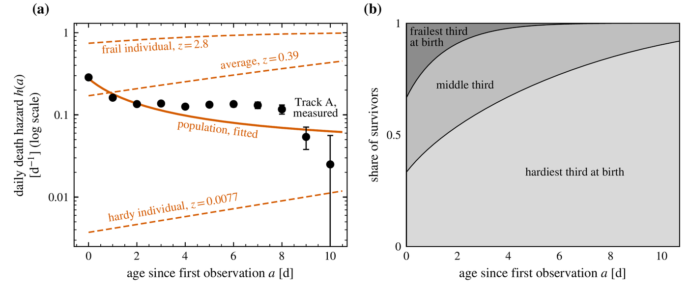
How a population can look ageless while every member ages. Left: the registry’s measured daily death rate (points) against the frailty model fitted to it, in which one exponentially rising individual hazard (dashed lines, drawn for a frail, an average and a hardy group) is mixed over a gamma distribution of hardiness; the mixture’s hazard (solid curve, fitted with far-side matches averaged) falls with age as the points do, though it runs below them at ages 3 to 8. Right: the share of the survivors at each age that were born in the frailest, middle and hardiest thirds; within a few days the frail are nearly all dead and the hardy dominate. The population’s death rate falls because the frail die early, while each surviving group’s own risk keeps rising. (Figure 2 of the sunspot paper.)
The sign of $B$ holds under every area form, every frailty shape and both far-side conventions fitted; its size varies, from +0.042 to +0.247 per day across those choices. An independent catalog from the Debrecen Observatory reproduces the age term. False deaths could mimic aging, since a small dying group is easy to lose; but simulated populations with no aging, pushed through the observing network’s measured loss rate, never came close to the measured slope. And the published decay laws, each converted into a death-risk law under three stated bridging assumptions, all fail against the registry. The authors add that a rejection applies to a law in the form they tested, not necessarily to the mechanism behind it, and that their study is a measurement made on the catalogs and does not claim that any published lifetime study is wrong.
The aging rate over the solar cycle
The Sun’s spot production rises and falls in a cycle of about eleven years, and near each maximum the magnetic field at the poles changes sign. The aging rate follows this cycle. In fits that the authors note were made outside the study’s original design, the age slope is enhanced inside a window that opens near each cycle maximum, as the polar field reverses (figure below). The enhancement has amplitude $k = 0.210 \pm 0.034$ per day, more than doubling the slope at maximum, and fades with an e-folding time of 2.25 ± 0.42 years, about as fast as the sunspot number itself declines.
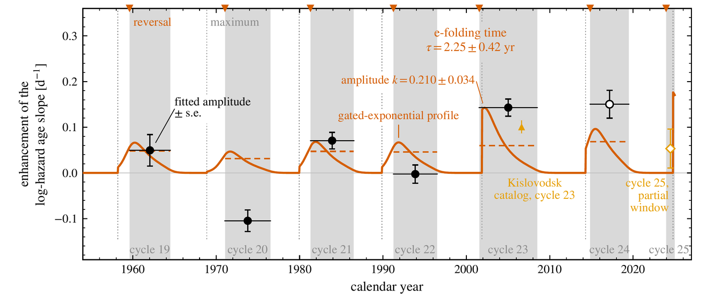
Cycle-by-cycle enhancement of the aging rate. For each cycle since 1954 the point is the fitted increase in the age slope inside that cycle’s window (gray band, opening at the polar-field reversal and closing at the next minimum), and the orange curve is the shared profile fitted to all of them: a jump near maximum that decays over about two years. The amplitude differs from cycle to cycle; cycle 20 is negative, cycle 24 (open) depends on the estimator, an independent catalog confirms cycle 23 (gold triangle), and cycle 25’s window had only begun (gold diamond). Aging runs faster for a couple of years after each cycle maximum, by an amount that varies between cycles. (Figure 6 of the sunspot paper.)
The amplitude of the enhancement varies from cycle to cycle. Cycle 20’s increment is negative under every estimator tried. Cycle 24’s depends on the estimator and comes out mildly negative on an independent catalog from the Kislovodsk mountain station, which nonetheless replicates the cycle 23 enhancement at seven to nine standard deviations. The window’s form was revised once after cycle 25 began, so cycle 26 will be the first test of the profile on a cycle that played no part in building it.
The eroding root
A rising risk at fixed visible state means that whatever destroys a group keeps some internal record of its age. The authors tested, in explicit mathematical form, six published mechanisms, seventeen aging mechanisms of their own, and roughly fifty candidate drivers and carriers of the cycle modulation. The data establish none of them. One is not eliminated, and the paper develops it as a physical hypothesis consistent with the measured law, and no more than that: a group would die when turbulent erosion thins its subsurface magnetic root past a breaking point.
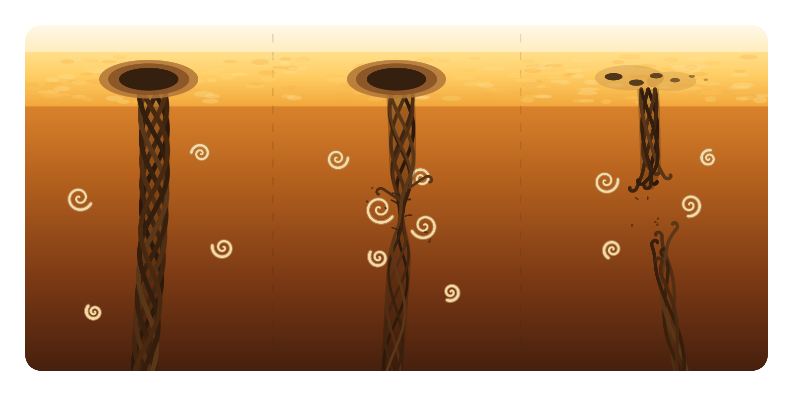
The one hypothesis the tests do not eliminate, drawn as a cartoon. From the surface the spot looks the same on each day, while convective eddies wear away the magnetic root that anchors it below; the group dies on the day a blow exceeds what is left. This mechanism would produce the pattern found in the registry: at equal size and hardiness, the older group is the likelier to die. (Site illustration of the hypothesis the paper draws schematically in its Figure 7; no data.)
In the eroding-root picture a group is the visible top of a bundle of magnetic flux, most of it below the surface, held at some anchoring depth by magnetic tension. Let $M$ be the margin, the flux connected at the anchor beyond the least that can hold the bundle, with value $M_0$ at emergence. Suppose eddies at that depth strip flux away steadily, so that $M(a) = M_0 - c\,a$. Suppose further that rarer, stronger blows arrive at random at a rate $\nu$, with strengths $\Phi$ exponentially distributed about a mean $\Phi_*$. The group dies at the first blow stronger than the margin that remains, so its hazard at fixed area is the rate of such blows (with $M_{0,i}$ the margin group $i$ is born with):
$$h_i(a) \;=\; \nu\,\Pr\big[\Phi \gt M(a)\big] \;=\; \nu\, e^{-M(a)/\Phi_*} \;=\; \nu\, e^{-M_{0,i}/\Phi_*}\, e^{B a}, \qquad B = \frac{c}{\Phi_*}.$$The risk rises exactly exponentially with age while margin remains, which is the factor $e^{Ba}$ found in the fits to the registry, and the prefactor $e^{-M_{0,i}/\Phi_*}$ plays the part of the frailty $z_i$: groups born with thin margins die first. The construction is borrowed from the Strehler–Mildvan theory of mortality (1960), and the exponential rise it produces is Gompertz’s 1825 law of human mortality. If the steady erosion removes about one blow’s worth of flux per convective turnover time $\tau_c$, then $B \approx 1/\tau_c$. A mixing-length estimate low in the convection zone gives $\tau_c \approx 3.5$ days, or $1/\tau_c \approx 0.29$ per day, the order of the fitted slopes, though that is under the fastest turnover-time convention in use and the conventions differ by a factor of three to five. The layers just below the surface overturn in hours, far too fast to match the fitted slope. The cycle modulation would then tie the root to the Sun’s global field, though the paper identifies no specific agent for it.
The authors stress that identifying the fitted rate with a turnover rate at an anchoring depth is an assumption, and that the depth is not measured. As first derived, the eroding-root hazard form also fits worse than the best unconstrained hazard shape by more than the decisive margin; under each far-side convention the shortfall comes from a single constraint of its premise, and with that constraint relaxed the form matches. Observational tests of the hypothesis exist or are scheduled: far-side imaging to follow groups past the limb, helioseismic imaging beneath groups of known age (under an eroding root, of two groups of equal area the older should look weaker below the surface), and Solar Orbiter’s high-latitude passes from 2029, in time for cycle 26.
On other stars, spot regions die without aging
On other stars, outside a handful with Doppler or transit maps, a dark region appears only as a small dip in brightness that recurs once per rotation until the region is gone. The companion paper calls a dip followed from rotation to rotation a spot feature, most likely several spots or groups blended at one longitude. The sample is 509 heavily spotted dwarfs observed by the Kepler and TESS space telescopes: Sun-like G and K stars, cooler and smaller early-M dwarfs, and 37 stars past the fully convective boundary, the mass below which a star has no radiative core and convects throughout. On these stars the authors tracked 10,051 features from birth to death and, to the roughly 6,500 of them on 260 stars that enter the fits, fitted the same kind of censored likelihood, with dip depth at birth in place of area and one frailty per star.
Starspot features give the opposite result from sunspot groups: at fixed birth depth, within a single star, a feature in its tenth rotation is at the same risk of dying as one in its third. On the G–K dwarfs the fitted age slope, 0.0056 per rotation, is consistent with no aging, and injected aging of 0.05 per rotation would have been detected. The solar rate on these stars’ rotation clock would be about 35 times that bound. On the early-M dwarfs the bound is a less secure 0.12. Median lifetimes run four to seven rotations across the samples and estimators, with the caveat that the tracking cannot follow a feature much beyond six or seven. For lifetimes the tracking can follow, the clock is the star’s rotation: across 438 Kepler stars the median lifetime $L$, in days, follows the rotation period $P$, in days, alone:
$$L \;=\; 10^{0.868}\,P^{\,0.828}\ \text{days}.$$The exponent’s 95% interval runs from 0.767 to 0.887 (figure below). Activity on cool stars is usually organized by the Rossby numberthe rotation period divided by the convective turnover time, the time a parcel of gas takes to rise and sink once in the star’s outer layers; activity indicators across cool stars line up best against this ratio, the period divided by the convective turnover time. Substituting it for the period loosens the fit for each of five published turnover scales, in every one of 10,000 resamples. Past the fully convective boundary the smaller TESS sample also shows a flat hazard and lifetimes proportional to the period, though there the simulations can neither bound aging nor identify the clock.
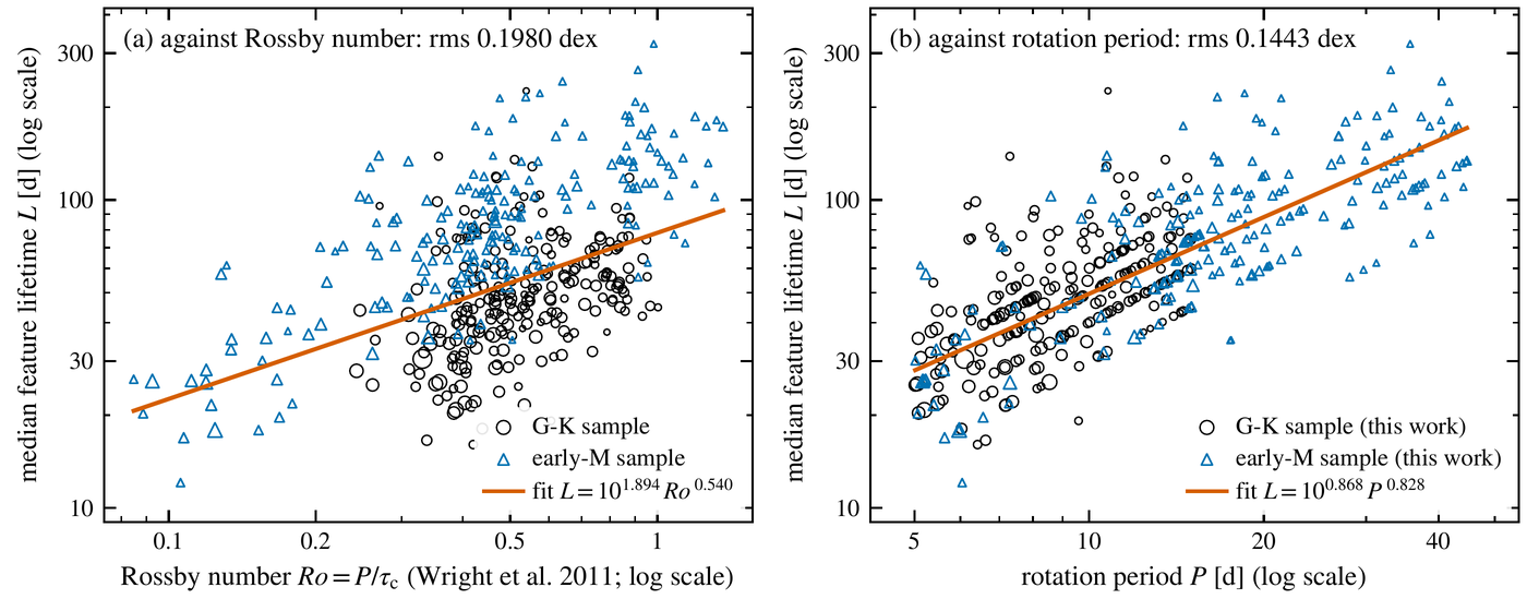
Which clock sets a starspot feature’s lifetime. Each symbol is one Kepler star’s median feature lifetime in days, circles for G–K dwarfs and triangles for early-M dwarfs, sized by its number of recorded deaths, plotted against the Rossby number (left) and against the rotation period alone (right), each with its fitted power law. The two spectral classes separate on the left and merge into one band on the right, where the scatter about the line is 0.144 dex against 0.198 (a dex is a factor of ten). Feature lifetimes follow the rotation period, growing as $P^{0.828}$, more closely than they follow the Rossby number that organizes other activity indicators, for each of the five turnover scales tested. (Figure 3 of the starspot paper.)
The Sun would not make it into the stellar sample, since its variability falls below the selection cut. Forward-modeled as a Kepler target it yields fewer than two trackable features per year of solar maximum and at most 13 in any four-year window, against the fifty a survival fit needs. The authors argue that the two results need not conflict if a light-curve feature is read as the stellar counterpart of a sunspot nest, a site where new spot groups emerge again and again. In a model of a site fed new groups at a steady rate, the site’s hazard settles to a constant once it is older than one or two member lifetimes, however the members age. On the Sun, where nests can be identified directly, they show no aging, in a test sensitive only to strong aging, while the groups inside them age.
The reconciliation of the solar and stellar results is not complete. No feeding configuration the authors tested reproduces the flat stellar hazard together with the observed lifetimes and depths: complexes built from aging solar-law groups still show aging through the analysis, and so does the one configuration tried with memoryless members. Either stellar features are fed faster, by shorter-lived groups, than scaled-up solar groups would supply, or the solar death law does not extrapolate to spots far larger than the Sun’s. Doppler imaging of one heavily spotted dwarf, rotation after rotation, would settle which.
The papers
- Demography of sunspots: aging, and death by turbulent erosion? (PDF) — Matthew D. Schwartz (Department of Physics, Harvard University) and Cecilia Garraffo (AstroAI, Center for Astrophysics | Harvard & Smithsonian); the version hosted here is marked preliminary. In this solar study the authors build the life table of sunspot groups from the Greenwich and USAF/NOAA registry, measure the age term in the groups’ death hazard and its variation over the solar cycle, and develop the eroding-root hypothesis.
- Starspot regions die without aging from G dwarfs to the fully convective boundary (PDF) — Matthew D. Schwartz and Cecilia Garraffo; the version hosted here is marked preliminary. In this companion study the authors apply the same analysis to spot features in Kepler and TESS light curves and find a flat hazard and lifetimes that follow the rotation period.
Supplementary material
For the solar study the authors state that code and derived data will be deposited in a public repository on acceptance and are available on request until then. The starspot paper comes with machine-readable tables of its 516 selected stars and 10,051 features, released with its target lists and code. Hosted on this site:
- sunspot-evaluate.py — Python (numpy, scipy): rebuilds the life table with a Turnbull estimator under both handlings of the broken records, refits five parametric survival families and the joint hazard models in area, age and frailty on the 25,883 birth-observed histories, and prints each recomputed value beside the paper’s printed one (the daily hazards at ages 0–10, the age slope $B=+0.1839$ per day, the area exponent $-1.153$, the age term’s AIC margin of 601.5), exiting nonzero on any mismatch;
--checkadds two controls that must fail. A full run takes under a minute. It reads the three data slices below from its own directory and verifies their checksums before use. - histories_A.json.gz — the 25,883 interval-censored lifetimes under the conservative handling of broken records, in which histories are never joined across the far side and every limb exit censors.
- histories_B.json.gz — the 24,489 lifetimes under the rotation-matched handling, in which records are joined across the far side when the rotation-predicted return matches.
- area_paths.json.gz — the daily corrected whole-spot area paths of the 25,883 birth-observed groups (95,468 group-days). All three slices are threaded from the Hathaway compilation of the Royal Greenwich Observatory (1874–1976) and USAF/NOAA (1977–2024) daily group catalog under the paper’s 14-day gap rule.
References
| B. Gompertz, On the nature of the function expressive of the law of human mortality, and on a new mode of determining the value of life contingencies, Phil. Trans. R. Soc. Lond. 115 (1825) 513 | the exponentially rising law of human mortality that the eroding-root hazard reproduces |
| M. N. Gnevyshev, On the nature of solar activity, Izv. Glav. Astron. Obs. Pulkove 16 (1938) 36 | decay at a rate set by present size, the origin of the lifetime–area law |
| H. W. Newton and M. L. Nunn, The Sun’s rotation derived from sunspots 1934–1944 and additional results, Mon. Not. R. Astron. Soc. 111 (1951) 413 | the rotation law used to match eastern reappearances to western exits |
| M. Waldmeier, Ergebnisse und Probleme der Sonnenforschung, 2nd ed., Geest & Portig, Leipzig (1955) | with Gnevyshev, the constant-rate decay tradition and $\tau = \alpha A_{\max}$ |
| B. L. Strehler and A. S. Mildvan, General theory of mortality and aging, Science 132 (1960) 14 | a declining reserve meeting random blows; the construction the eroding-root hazard borrows |
| G. W. Simon and R. B. Leighton, Velocity fields in the solar atmosphere. III. Large-scale motions, the chromospheric network, and magnetic fields, Astrophys. J. 140 (1964) 1120 | spot death by erosion from the surrounding convection |
| B. W. Turnbull, The empirical distribution function with arbitrarily grouped, censored and truncated data, J. R. Stat. Soc. B 38 (1976) 290 | the estimator that extracts a survival curve from interval-censored records |
| J. W. Vaupel, K. G. Manton and E. Stallard, The impact of heterogeneity in individual frailty on the dynamics of mortality, Demography 16 (1979) 439 | frailty: a fixed, unobserved multiplier on each individual’s hazard |
| K. Petrovay and F. Moreno-Insertis, Turbulent erosion of magnetic flux tubes, Astrophys. J. 485 (1997) 398 | the quantitative theory of turbulent erosion of a spot’s flux tube |
| N. J. Wright, J. J. Drake, E. E. Mamajek and G. W. Henry, The stellar-activity–rotation relationship and the evolution of stellar dynamos, Astrophys. J. 743 (2011) 48 | the rotation–activity relation; its turnover times give the Rossby number plotted above |
| H. A. C. Giles, A. Collier Cameron and R. D. Haywood, A Kepler study of starspot lifetimes with respect to light-curve amplitude and spectral type, Mon. Not. R. Astron. Soc. 472 (2017) 1618 | starspot decay timescales from Kepler light-curve autocorrelation, by spectral type |
| K. Namekata, H. Maehara, Y. Notsu, S. Toriumi, H. Hayakawa, K. Ikuta, S. Notsu, S. Honda, D. Nogami and K. Shibata, Lifetimes and emergence/decay rates of star spots on solar-type stars estimated by Kepler data in comparison with those of sunspots, Astrophys. J. 871 (2019) 187 | individually tracked spots on Sun-like Kepler stars, with lifetimes rising with rotation period |
| D. H. Hathaway, Royal Greenwich Observatory and USAF/NOAA sunspot group records, 1874–present, solarcyclescience.com/activeregions.html (2024) | the compiled daily group catalog from which the registry and the data slices above are threaded |