Feynman diagrams (quantum field theory)
The content on this page was written by AI under human supervision.
Feynman diagrams are the little line drawings physicists use to compute what happens when particles collide, and every diagram stands for an integral. The hardest of those integrals have resisted computation for decades, because their answers live on ever deeper geometry: polylogarithms, then elliptic curves, then K3 surfaces and Calabi–Yau manifolds. The three papers behind this page present an automated bootstrap that reads the geometry off the diagram, eliminates almost every candidate answer with exact consistency constraints, and pins down the few constants that remain, accepting a result only when it reproduces independent values that entered no step of its derivation, to thirty digits or more. Thirty frontier integrals are carried from diagram to checked closed form: fifteen blind reproductions of known results, and fifteen new, several of them explicitly left open in print.
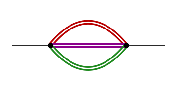
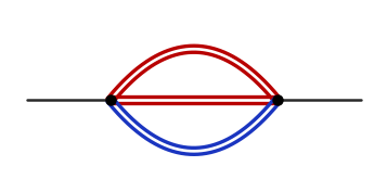
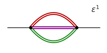
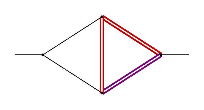
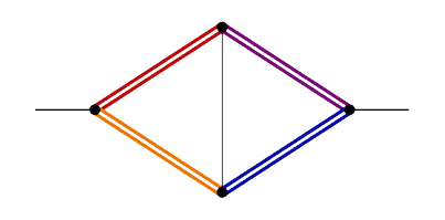
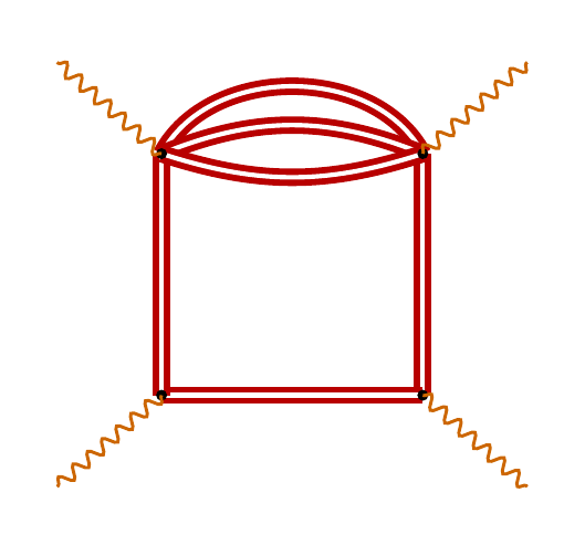
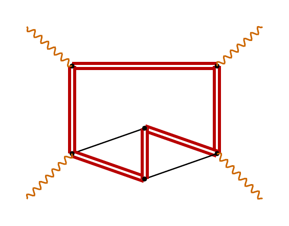
The 30 diagrams. Click each for details.
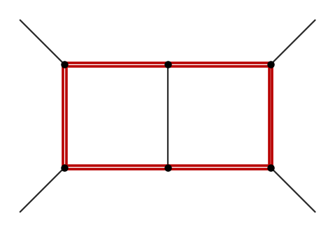
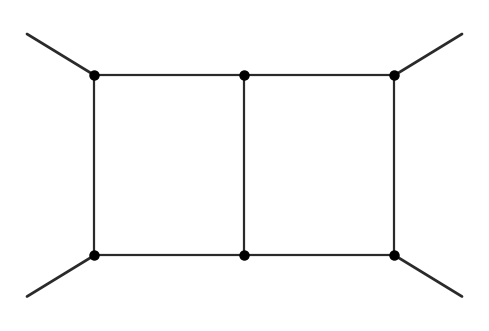
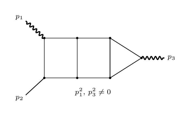
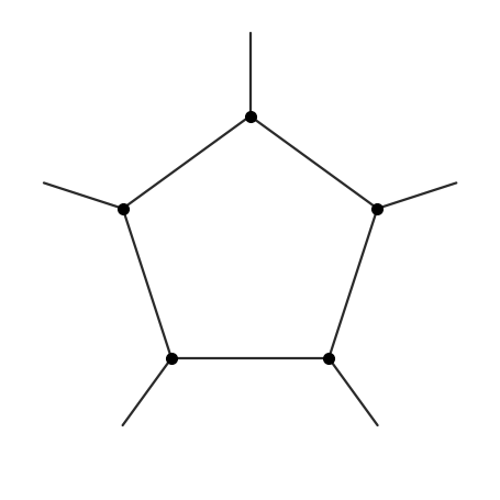
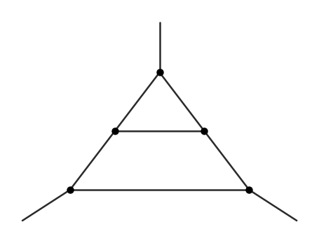
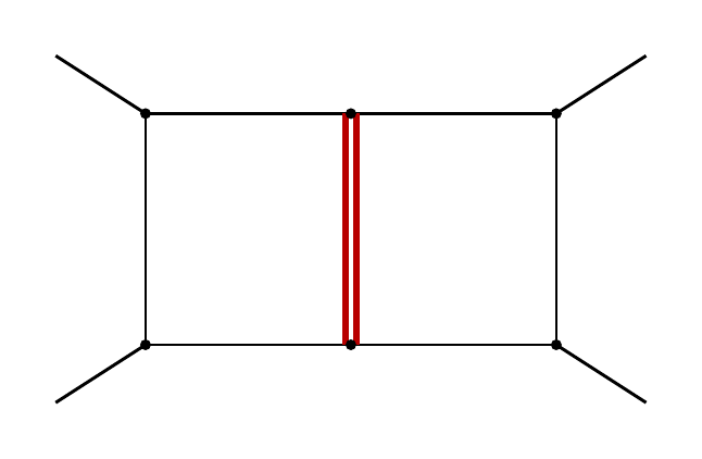
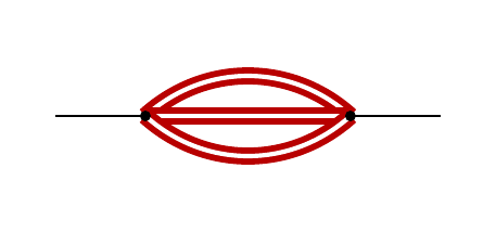
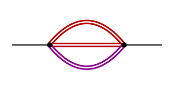
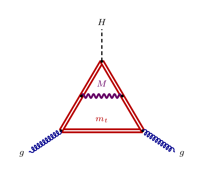
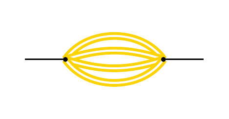
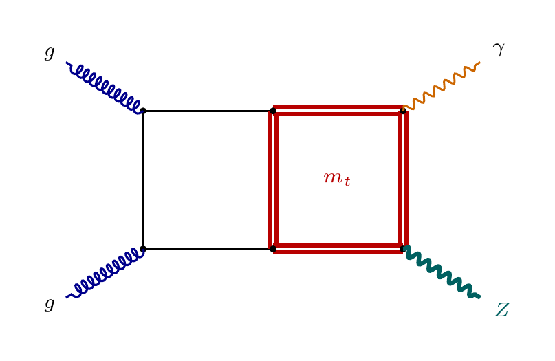
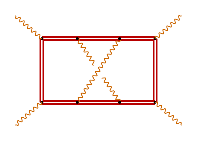
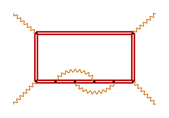
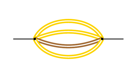
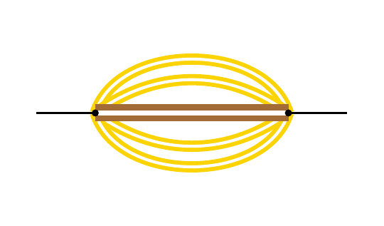
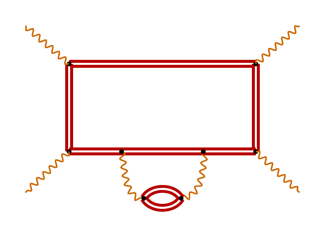
Summary
- Thirty frontier Feynman integrals, diagram to closed form: fifteen blind reproductions of known results and fifteen new, each with an explicit formula and a standalone evaluator anyone can run, agreeing to thirty digits or more (most elliptic cases at 90 to 160) with independent values withheld from every step of the derivation.
- The W-pair branch left open in print is solved: the nonplanar branch of two-loop W-pair production with exact top-quark mass carries 76 master integrals, 23 with no previous computation; the solution agrees to 37 digits with independent values never used in any fit, improving to 57 as the evaluator’s precision is raised.
- Some answers are genuinely new numbers: the ice-cream cone’s boundary constant is proven to lie outside every classical ring tested, and it is written out as an explicit convergent integral rather than a string of digits.
- New geometry sits at the thresholds: the sunrise degenerates at its threshold through a non-semistable Type III fiber, the first documented for a Feynman elliptic surface, and the new threshold constants lie in classical rings; at four loops, the lemniscatic period enters the banana tower for the first time.
- Two of the results are impossibility proofs: the crossed light-by-light box’s top integral has no polylogarithmic form in any basis, and the banana tower cannot yield the hoped-for non-CM period.
- The pipeline is public: a language model working under human direction consolidated the community’s engines into one open toolkit (Mathematica-free on the critical path), added roughly a hundred purpose-built tools, and computes no digits itself; the acceptance test never depends on its judgment.
Non-technical summary
Nearly everything physicists can predict about colliding particles comes, in the end, from Feynman diagrams: the small line drawings, named for the physicist Richard Feynman, in which particles fly in, trade other particles back and forth, and fly out. A diagram looks like a cartoon, but it is really an instruction. Attached to every diagram is an integral — a continuous sum over all the ways the particles inside the drawing can share energy and momentum — and the number that integral produces is that diagram's contribution to the prediction. The trouble comes from diagrams with closed loops, in which particles briefly appear, circulate, and vanish again, as quantum mechanics allows. Every added loop makes the prediction more precise, and the integral dramatically harder.

Figure 1. The same collision, drawn ever more finely. Each added loop sharpens the prediction and multiplies the difficulty of the integral.
Precision is how particle physics moves forward now. At the Large Hadron Collider, one path to discovering new physics is to measure a process very well, predict it equally well, and look for a discrepancy — and the bottleneck of the predictions is evaluating these loop integrals. The integrals have a second constituency in pure mathematics: the hardest ones involve some of the deepest objects in modern geometry and number theory, and integrals of exactly this type appear in problems as far afield as the scattering of black holes and random walks on a crystal lattice.
Progress stalled for decades because the answers climb a ladder of geometry. The easiest integrals evaluate to logarithms and their iterated cousins, and decades of work turned that class into settled, nearly push-button methodology. But give the particles running around a loop enough mass and energy scales, and the geometry hidden inside the integral changes: a core piece of the calculation no longer traces out a sphere but a torus — the surface of a donut, which mathematicians call an elliptic curve — and the answer needs the donut's own special functions, for which there is no complete calculus. More loops push the donut into its higher-dimensional cousins, the K3 surfaces and Calabi–Yau manifolds, where even fewer rules exist. The emblem of the difficulty is the sunrise diagram, a modest drawing of massive particles traveling together from one point to another: it held out for decades, and when it finally was solved it was solved several times over, in different mathematical languages, with translation between the solutions a research problem in its own right. Each new integral at this frontier has, in practice, been a research paper of its own — and the community's software tools, individually excellent, were built by different groups, in different programming languages, behind different conventions.
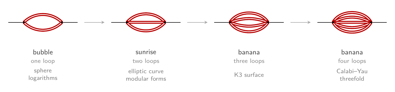
Figure 2. The banana tower. The same diagram gains one massive line at each rung, and the geometry underneath climbs with it — a sphere, then the donut, then the donut’s higher-dimensional cousins — each rung with fewer rules of calculus than the one below.
BootLoops attacks this frontier with two moves. The first is consolidation: a large language model (Claude, from Anthropic), working under human direction, rebuilt the community's best programs into one shared, open, tested toolkit, and wrote new tools to fill the gaps. A single operator can then hold the specialties that fragmentation kept apart: the physicist who sets up the problem, the mathematician who recognizes the functions, and the programmer who drives the software. The second move is the bootstrap itself — physics slang for pulling an answer up by its own consistency rather than grinding through the integral. The geometry can be read off the diagram alone, and it fixes the entire family of functions the answer can possibly be built from. Consistency requirements then eliminate almost every candidate, the way a crossword's grid and a few crossing words eliminate almost every letter, until only a handful of unknown constants survive to be pinned against extremely precise numerical evaluations; where a fit provably cannot work, the machinery instead solves the integral's own differential equation, under the same rules. And every result must pass one test before it counts: it has to reproduce independent evaluations that entered no step of the derivation — digits no fit ever saw — to thirty decimal places or more. A wrong formula can fit the points used to build it; it cannot match that many fresh digits by luck.
The outcome is a portfolio of thirty of these frontier integrals, each carried from the drawing to a checked formula. Nearly half rederive known answers, several among the hardest in the published literature, recomputed with those answers withheld from every step and compared only at the end — all of them came back right, and the new results stand on that validation. The rest are new, several explicitly left open by the papers that came before, among them a missing piece of the prediction for how often colliders produce pairs of W bosons. Some of the answers turned out to be genuinely new numbers: constants proven to be on no mathematician's list, delivered as explicit convergent integrals rather than digit strings. The geometry held a surprise of its own — at the exact collision energy where the particles circulating in a loop can first materialize as real particles, the donut underneath the sunrise degenerates in a fashion never before documented for a Feynman diagram. And twice the discovery was a proof that a thing cannot be done: a simpler formula that provably does not exist, and a hoped-for new kind of number that the arithmetic of the underlying surfaces forbids. Every result comes with an explicit formula and a small program anyone can run, and the papers state plainly what remains out of reach: the next geometry up — curves with more holes than the donut has — calls for mathematics that does not yet exist in usable form.
Introduction
Ask a theorist what happens when two protons collide at the Large Hadron Collider and the answer begins with line drawings: particles enter, split, circulate, and rejoin, sketched as Feynman diagrams. The drawings are working notation. Quantum field theory — the framework underlying all of particle physics — makes almost no predictions in closed form; it offers instead a controlled approximation, the answer written as a series of ever-smaller corrections, and the diagrams are the bookkeeping of that series. Each diagram stands for a definite multi-dimensional integral, its Feynman integral, taken over the momenta of the particles circulating inside it; the closed loops set its loop order, and every loop adds one more order of accuracy in the prediction and a steep jump in difficulty. When a collider measurement is compared against theory, the theory side is, at bottom, a sum of Feynman integrals.
Evaluating those Feynman integrals is the computational bottleneck of the precision program in collider physics. At low loop order they are under control. At the frontier, where more loops, internal masses, and extra kinematic scales pile up, each integral has traditionally been a research project of its own, and the hardest have resisted every generation of methods for decades. The reason is a shortage not of computing power but of mathematics: harder diagrams demand a ladder of ever deeper function classes — first ordinary logarithms, then polylogarithms, then functions on elliptic curves, and finally periods of K3 surfaces and Calabi–Yau manifolds, objects from the far end of modern algebraic geometry.
The bottom rungs of the ladder are a settled story, told with names and dates in the next section. At one loop the problem was solved as a class in 1979; beyond it, two structural discoveries organize everything — the thousands of distinct integrals any one process generates all reduce to a small basis of master integrals, and the masters obey differential equations in the collision energies that, in the right basis, reduce order by order to linear algebra plus a boundary value. Twenty years of this turned polylogarithmic Feynman integrals from exotic research problems into core knowledge — polylogarithms being the functions built from the logarithm by repeated integration, the first of them the dilogarithm $\mathrm{Li}_2(z)=\sum_{n\geq 1} z^n/n^2$. (Because the integrals harbor infinities, they are computed in $d=4-2\varepsilon$ spacetime dimensions and delivered order by order in $\varepsilon$: the epsilon expansion in which every result in this subject is expressed.)

Figure 3. Landmarks of the multi-loop frontier, in time. Above the axis, the polylogarithmic line of advance, from the one-loop vertex behind the electron’s $g-2$ to the two-loop five-point frontier. Below it, in red, the sunrise ladder: the same two-point topology gaining one massive line per loop, with the year each rung fell — the elliptic sunrise in 2005, the K3 banana in 2015, the Calabi–Yau banana in 2023. The 2026 entry is this program: thirty frontier integrals from diagram to closed form, the ice-cream cone drawn here among them, each checked against independent values withheld from its derivation.
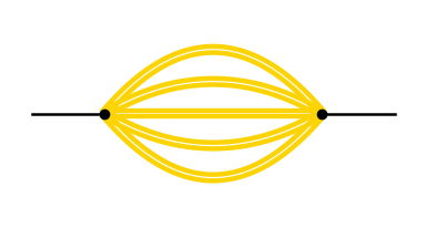
Above the polylogarithmic rungs the textbook ends. The controlling geometry of a Feynman integral is its maximal cut, the skeleton integral obtained by forcing every internal particle onto its mass shella particle is on its mass shell when its energy and momentum obey the relation $E^2=p^2+m^2$ that a real, observable particle satisfies; particles inside a loop need not; the shape the maximal cut traces out determines which functions the full answer can contain. For the integrals of the previous paragraph that shape is a sphere, and spheres give polylogarithms. But the moment the maximal cut lands instead on a surface with a hole (an elliptic curve, geometrically a torus), the answer becomes an elliptic polylogarithm, an iterated integral of modular forms, or a period of a K3 surface or Calabi–Yau manifold, higher-dimensional generalizations of the elliptic curve — and every automated method that made polylogarithms routine fails at once. The archetype is the two-loop sunrise, a diagram in which a particle splits into three massive particles that recombine: it went unsolved for more than four decades, and once solved it was solved at least five times, in five different function languages, with no dictionary between the solutions. Stacking more loops into the sunrise produces the banana graphs, and the geometry escalates rung by rung: a K3 surface at three loops, a Calabi–Yau $(L-1)$-fold at $L$ loops.
A harder question underlies the fragmentation: what should it mean to have computed a Feynman integral at all? Numerical machinery can hand you hundreds of digits at any single kinematic point, but a value is not a function — a string of digits comes with no function space, no branch points, no way to expand near a threshold. Solving means identifying the functions, and an identification needs a test that a wrong answer cannot pass: a fit to the wrong function space will happily reproduce the points it was fitted to and then fail everywhere else. The check that counts is agreement, to dozens of digits, with independent values withheld from every step of the derivation.
One response has been developing in the amplitudes community for over two decades: the bootstrap, the strategy of pinning an answer down from the constraints it must satisfy — its allowed singularities, its symmetries, its behavior at special points — rather than by brute-force integration. The pieces of a working bootstrap all exist in the community's toolbox: symbols and canonical forms, large systems of differential equations, high-precision numerics, integer-relation fits that turn long strings of digits into exact constants. Assembling them for a single frontier integral has demanded exactly what the fragmented community could not routinely supply: one person working as physicist, mathematician, and programmer across software written in five languages. The three papers this page is built on start from the observation that the current generation of large language models can play all three roles at once. The result is an automated system called BootLoops, presented in three parts: a method paper that builds the machine, a geometry paper that follows it up the elliptic and Calabi–Yau ladder, and a portfolio paper that records thirty frontier integrals carried from diagram to checked closed form. Everything below hangs on the question those papers were written to answer: can the hardest Feynman integrals be computed automatically, in explicit closed form, and checked against digits that no fit ever saw?
Current knowledge
The one-loop problem was solved as a class. In 1979 Passarino and Veltman showed how to reduce any one-loop amplitude to a small basis of standard integrals, and every one-loop answer is built from logarithms and dilogarithms — the first members of the family of polylogarithms, the iterated generalizations of the logarithm.
Beyond one loop, brute force fails, and physicists built an assembly line instead. Integration-by-parts identities, dating to Chetyrkin and Tkachov, relate the thousands of integrals in a diagram family to one another; in 2000 Laporta's algorithm ordered those identities into solvable linear systems, turning reduction into an industrial process whose output is a short list of master integrals. The masters satisfy coupled differential equations in the kinematic variables, so computing a family becomes solving that system from one known boundary point — Gehrmann and Remiddi's two-loop four-point calculation of 2000 marks the arrival of this machinery at the frontier of its day. The mathematics that organizes the answers largely came from outside physics: Chen's iterated path integrals and Goncharov's multiple polylogarithms predate most of the physics that now uses them. In 2010 Goncharov and collaborators distilled the symbol — a fingerprint recording a polylogarithmic function as the sequence of logarithmic arguments it is built from — and in 2013 Henn observed that a good choice of master basis renders the differential equations canonical: $\varepsilon$-factorized, solvable order by order as linear algebra plus a boundary value. That one observation, more than any other, is why the polylogarithmic sector is automated at all. By 2016 the machinery reached two-loop five-point kinematics (Gehrmann, Henn and Lo Presti), and the material has settled into lectures and textbooks — in the geometry paper's words, “a physicist computing a polylogarithmic amplitude today finds mature tools at every step and rarely needs the original mathematics literature at all.”
Numerics kept pace. Liu and Ma's auxiliary-mass-flow method (the AMFlow package, 2022) delivers the value of essentially any master integral to hundreds of digits at any chosen kinematic point; sector decomposition, an older and fully independent technique, integrates the parametric representation directly. But a number at one kinematic point reveals nothing about what kind of mathematical object the answer actually is.
The real trouble begins when the geometry underneath an integral changes. Add enough internal masses or scales and the maximal cut's sphere becomes a torus — an elliptic curve — and the answer leaves the polylogarithms entirely: it must be built instead from the torus's periods, the two numbers measuring a trip once around each of its loops. The two-loop sunrise resisted polylogarithmic evaluation from Sabry's calculation of 1962 until the first analytic elliptic evaluation by Laporta and Remiddi in 2005, forty-three years later. The tower keeps growing: the banana graphs place the maximal cut on a K3 surface at three loops and on a Calabi–Yau manifold beyond, with the traintrack and fishnet families supplying infinite towers past those; in 2023 Pögel, Wang and Weinzierl carried the $\varepsilon$-factorized differential-equation technology up to the Calabi–Yau banana, a landmark of the direct-computation line. But on this frontier the three pillars of the automated pipeline all fail at once: no algorithmic canonical-form theory exists beyond the polylogarithms, no finite symbol calculus, and the reduction and numerical machinery is blind to the function class it is working over. Answers exist, but in no standard language — the equal-mass sunrise alone has been solved in five function vocabularies, from elliptic dilogarithms to iterated integrals of modular forms to dispersion relations — and nearly everything known is anchored at special points singled out by the mathematics, where mirror-symmetry or modular-form techniques apply, rather than at the physical thresholds where particle-production channels open.
A second obstacle was quieter: the community's software did not work together. The method paper surveys the stack and counts twenty-three excellent public packages covering the six elements of a complete pipeline, spread across five programming languages plus two computer-algebra ecosystems: nine are Mathematica-native, making a Wolfram license a de facto prerequisite for roughly half the stack, and four separate engines implement Laporta's algorithm, interchangeable in principle and incompatible in practice. Even the ideas travel slowly. The Landau equations — the classical conditions, as old as the analytic S-matrix, that locate an integral's singularities — became push-button only recently, through Mizera and Telen's Landau discriminants (2021) and the packages PLD.jl (2023) and SOFIA (2025), with the packages emerging from a different community (computational algebraic geometry). The paper states the cost plainly: “A community whose tools do not circulate pays for every result twice: once to build the method, and once more in every group that reconstructs it by hand for want of knowing it existed.”
The word bootstrap in amplitudes names a strategy rather than a single method: instead of integrating, write down the space of functions the answer could possibly be, then cut that space down with everything known about the answer's analytic structure until only one candidate survives. For polylogarithmic amplitudes the tradition is mature; Morales, Spiering, Wilhelm, Yang and Zhang bootstrapped elliptic Feynman integrals at the level of the symbol, and no Calabi–Yau bootstrap appears in the record at all. The two methods this program directly extends both stopped at the elliptic curve. The Landau bootstrap of Hannesdóttir, McLeod, Schwartz and Vergu constrains an integral from its singularity locus and the local behavior nearby, without committing to a function class; analytic regression, by Barrera, Dersy, Husain, Schwartz and Zhang, samples an integral to hundreds of digits and uses integer-relation fits — algorithms that recognize exact constants inside long strings of digits — to pin down the answer's coefficients, with the elliptic case explicitly deferred: without an enumerable function space, the fit has no well-posed target.
When this program began, then, the polylogarithmic sector was a solved industrial process, but from the elliptic curve onward the answers had no agreed-upon language, the bootstrap had no function space to search, and integrals that collider predictions were waiting on stayed open in print: the nonplanar branch of two-loop $q\bar q \to W^+W^-$ with exact top-quark mass, closed elliptic masters for $gg \to Z\gamma$, the five-point integrals bottlenecking $W/Z$-plus-jet predictions (the open list is collected in the portfolio paper). Every element of a complete pipeline existed somewhere, in print, at high quality; the composition did not. The next section describes how this program assembled all of it in one place.
BootLoops approach
Every ingredient of a modern Feynman-integral calculation existed as public software before this program began; the missing piece was composition, not a new theorem. The premise of the method paper, Automated computation of Feynman integrals with BootLoops, is that a large language model can hold all three of the required specializations at once — in the paper's words, "a strong physicist to set up the problem, a great mathematician to recognize the functions, and an effective programmer to drive the tools." BootLoops is the harness built on that premise, and its first job was consolidation: the community's packages were ported out of their native languages into one uniform open toolkit in which no required step needs a Mathematica license — the singular-locus engine SOFIA rewritten in Julia, auxiliary mass flow running through a C++ port adopted after an audit, the Landau-bootstrap ansatz machinery rewritten as LandauBootstrap, with Kira and PLD.jl used as released. Around these the program wrote roughly one hundred purpose-built tools where no public equivalent existed, each documented in an online registry.
On top of the toolkit sits the method, which the papers call the hybrid bootstrap. It provides two routes to every integral. The constraint leg is the bootstrap proper: fix the space of functions the answer can live in, cut that space down with exact analytic constraints, and fit the little that remains against high-precision numbers. The integration leg is the classical route — reduce to master integrals, build their differential equations, solve them — carried as an equal alternative under the same acceptance rule. The bootstrap goes first where it applies because it is cheap; a decision layer routes an integral to the integration leg when the bootstrap provably cannot close it. Both legs descend from the two parent methods of the previous section — the constraint leg from the Landau bootstrap, the fit from analytic regression — and where the regression paper had no enumerable function space to aim at, the pipeline supplies that target from geometry.
The mathematical backbone is the differential-equation method in Henn's 2013 canonical normalization, in which the vector of master integrals $\vec g$ obeys a first-order system with $\varepsilon$ factored out completely:
$$ d\,\vec g \;=\; \varepsilon\, A\,\vec g \,, \qquad\qquad dA \;=\; A \wedge A \,.$$
Here $\vec g$ lists the master integrals, each normalized to uniform weight (the count of nested integrations — one for a logarithm, two for a dilogarithm), and $A$ is a matrix of differential forms in the kinematic variables: for polylogarithmic integrals $A = \sum_k A_k\, d\log \alpha_k$, where the $\alpha_k$ are the letters of the integral's alphabet, a finite list of algebraic functions recording every place the answer can have a branch point; on the elliptic and Calabi–Yau rungs the $d\log$ kernels are replaced by kernels built from the periods of the underlying geometry. Because $\varepsilon$ multiplies the whole right-hand side, the solution at each order is an iterated integral over these kernels — a sum of "words" spelled in the letters — so the function space becomes something one can enumerate. The second equation says the connection is flat: the iterated integrals must not depend on the integration path. In several variables that condition cross-links the entries of different words and becomes the single heaviest constraint in the program — for one three-loop crossed double box it cut the weight-four candidate space from 2401 words to 1166 before any other condition was imposed.
Every bootstrap closure then follows the same four steps.
- Step 1: find where the answer can be singular. The Landau equations locate the kinematic points where an integral can develop a singularity, delivered algorithmically by PLD.jl and SOFIA from the graph alone as the principal Landau determinant, whose irreducible factors are exactly the candidate letters — including letters no one would write down by hand, such as the quadratic $x^2 - 10x + 5$ for one two-loop three-point integral. In parallel, the maximal cut reveals the geometry the answer lives on: a sphere for polylogarithms, an elliptic curve one rung up, a K3 surface or Calabi–Yau manifold above that.
- Step 2: write down what the answer can be. The maximal cut also supplies the leading singularity, the prefactor that normalizes each master integral to uniform weight, and the answer becomes an ansatz, schematically $$ I \;=\; \mathrm{LS}(x) \sum_{w} c_w\, f_w(x)\,,$$ with the $f_w$ iterated integrals labeled by words $w$ in the alphabet and the $c_w$ unknown numbers — rational coefficients plus a handful of genuine boundary constants.
- Step 3: cut before you fit. Every available structural constraint is imposed before any numerics: the flatness condition above; the first-entry condition (only physical branch points can open a discontinuity); parity and Galois symmetry of the kinematics; residue and sum rules at special points; and the arithmetic of the ring the constants can live in. Together these collapse an unbounded function space to a residual of a few hundred to a thousand unknown numbers, small enough for a fit to pin.
- Step 4: fit the residual, then test it on digits no fit ever saw. Auxiliary-mass-flow numerics with Kira reduction generate high-precision samples of the master integrals; PSLQ and LLL — integer-relation algorithms that recognize the exact combination of candidate constants inside a number known to hundreds of digits — pin the residual coefficients. Then comes the acceptance test: the fitted form must reproduce independent values, at kinematic points withheld from every derivation step, to thirty digits or more. (A closure, in the papers' vocabulary, is an identification of the integral in explicit form that has passed this test.)
Both halves of the design, the analytic cuts and the numerical fit, are essential. A purely analytic closure is not demanded — the canonical-form theory that would permit one stops at the elliptic frontier, and insisting on it means waiting for mathematics that has not been invented. A purely numerical fit of an uncut ansatz is forbidden, because it is curve-fitting: with nothing constraining the space, the fit memorizes the sample points and predicts nothing.
The decision layer sits above the two legs. A geometry classifier reads the graph and returns the maximal cut's genus, its modular data, and a recommended route before any samples are computed. Its sharpest rule is the value-fittability criterion: an elliptic curve has two independent periods, and the maximal cut supplies the bootstrap with only the first; when a master integral's normalization involves only an algebraic function or a single global power of that first period, the fit of Step 4 can close it, but when the normalization mixes the two periods — through the quasimodular Eisenstein series $E_2$ — a value fit is provably impossible, not merely hard. Integrals in the second class are routed to the integration leg and solved by transporting the differential equation from an exactly known boundary, under the same thirty-digit acceptance, and the impossibility is proved as a theorem rather than left as a stalled run. Of the portfolio's thirty rows, twenty-four closed through constraints and fits and six through the integration leg, each of the six with a stated reason.

Figure 4. One procedure with two routes and a single test at the end. Reading from the top: reduction to master integrals and the singular-locus and cut-geometry analysis (Step 1) fix a canonical basis and the space of functions the answer can contain, and the analytic constraints cut the graded ansatz (Steps 2 and 3) before any number is computed. The value-fittability criterion then sends each master integral down one of two routes — a coefficient fit against high-precision values at sample points $x_a$ (Step 4, left), or, when a fit is provably impossible, transport of the $\varepsilon$-form differential equation from derived boundary data (the integration leg, right) — and both routes end at the same test: agreement to at least thirty digits at kinematic points $x_b$ that entered no fit. (The method paper’s Figure 1, with its equation references removed and its class labels A, B and C replaced by the terms used on this page.)
Before the pipeline was pointed at anything new, it was calibrated on the flagship example of both parent methods: the outer-mass double box of Caron-Huot and Henn. The twelve-letter alphabet was re-derived from the graph alone, with the published answer excluded from every step; the published constraint cascade — 20,736 raw ansatz terms cut to 161 — was reproduced exactly, by exact rational linear algebra in place of the original numerical step; and the fit closed from 24 sample points where the published protocol had used 200. The closed form then matched fresh values at four dedicated points, none of which entered any fit, to 39 digits, and both improvements carried forward to every new target.
The validation discipline is uniform across all three papers, and the method paper names it the BootLoops standard: an integral counts as computed only when three things exist. First, an explicit symbolic final form over a declared alphabet, in which every constant is either classical or defined by a written-out convergent integral. Second, a standalone evaluator — one script that reproduces the result at any kinematic point and any precision from arbitrary-precision arithmetic alone, with no loop-integral software behind it. Third, agreement with independent values withheld from the derivation — disjoint kinematic points, and where possible a disjoint kinematic region — to thirty digits or more, with every accepted digit vouched for by agreement between two runs at different precisions. Thirty is the floor; most elliptic rows clear 90 to 160 digits. The logic is a falsification test: a dimensionally regulated Feynman integral has one correct value at each kinematic point and each order in $\varepsilon$, so a $k$-digit match at points the fit never saw is a coincidence with probability of order $10^{-k}$ unless the form is the integral. An independent pass then reproduces each fit from scratch and confirms the result is stable when any single sample point is dropped; where possible the two numerical engines cross-check each other — sector decomposition (pySecDec) shares no machinery with auxiliary mass flow, which makes one a genuine cross-check of the other. Two caveats are stated alongside the standard: the papers report each closure in the tradition of Laporta's high-precision identifications — numerically overwhelming evidence, never a symbolic proof, and labeled as such — and the bootstrap itself is not claimed as a first; the narrower claim is a function-level pipeline that carries boundary constants, not only symbols, through an independent acceptance test.
One episode shows why the discipline earns its keep. When the harness first took up the nonplanar branch of two-loop $W$-pair production, configuration files inherited from the literature silently defined a different integral family — 98 master integrals instead of the true 76 — and every internal check (reduction, numerical oracle, and differential equation alike) stayed perfectly self-consistent on the wrong object. An audit of the graph's vertex structure caught the mismatch, and the lesson became a rule the pipeline now enforces: internal consistency proves nothing about identity, so the family is verified against the graph before anything else runs. The division of labor with the language model follows the same logic. The tools compute every number and every symbol; the model classifies the target, routes it, runs the tools, and assembles the result; nothing in the chain asks the model for a digit, and its judgment never touches acceptance — a fit either reproduces the independent values or it does not.
The method paper contains everything a reader needs to run this recipe on an integral of their own. The geometry companion, Bootstrapping elliptic and Calabi–Yau Feynman integrals, follows the same recipe from polylogarithms up the elliptic, K3, and Calabi–Yau rungs; the portfolio paper, Polylogarithmic, elliptic, and Calabi–Yau Feynman integrals from a hybrid bootstrap, and the Results below report what the recipe computed: thirty integrals end to end.
Results: the thirty-integral portfolio
The results of the portfolio paper come first: the thirty integrals, the new solutions and the blind reproductions behind them.
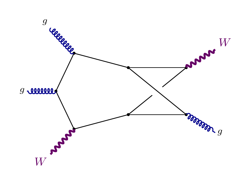
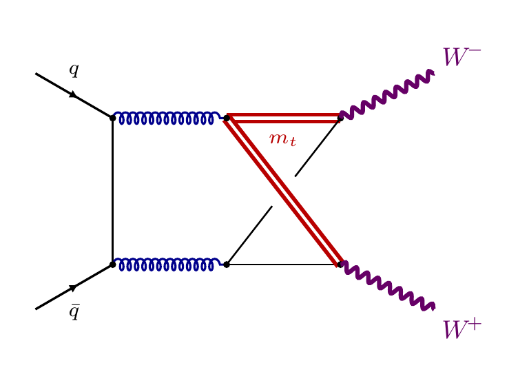
The W-pair branch the published calculation left open. When He, Zhang, Han, Jiang, Li and Wang published the two-loop master integrals for $q\bar q\to W^+W^-$ — quark–antiquark annihilation into a pair of W bosons, with the top quark's mass kept exact rather than approximated away — they computed the three planar branches of the problem and wrote that the fourth, the nonplanar branch $T_4$, was left to future work. The bootstrap solved it. The branch carries 76 master integrals, 23 of them with no previous computation, including a sector that lives on an elliptic curve appearing nowhere in the planar branches. The solution is an explicit symbolic form on a one-dimensional kinematic line, and all 79 components of its basis were compared against independent high-precision evaluations at points withheld from every step of the derivation: the worst component agrees to 37 digits when the evaluator runs at 40-digit precision, and to 57 digits when it runs at 60 — agreement that deepens with the requested precision, the behavior of an exact formula. No earlier computation of this branch has been found in the literature (the portfolio paper, row 35; the W-pair page).

Figure 5. The branch the published calculation left open. The nonplanar $T_4$ topology of two-loop $q\bar q\to W^+W^-$ with exact top-quark mass — thin lines massless, violet lines carrying the top mass $m_t$, wavy lines the on-shell $W$ bosons; the two propagators crossing without a vertex make it nonplanar. The three planar branches of this process were published by He, Zhang, Han, Jiang, Li and Wang, who left this branch open; it is solved here in explicit symbolic form — 76 master integrals, 23 with no previous computation, including an elliptic sector absent from the planar branches. (From the portfolio paper’s Figure 18.)
Two more collider bottlenecks, and a polylogarithmic box re-derived. Three further results bear directly on quantities experiments measure.
- Five-point integrals for WW/WZ-plus-jet. The two-loop five-point integrals with two massive external legs are a standing bottleneck for predicting a pair of vector bosons produced together with a jet. The planar families have been mapped, but the two non-planar families — 219 and 190 master integrals — remained open. The program determined their entire shared function space top-down, from the geometry of the diagrams alone, with no integration of differential equations and no numerical fitting: at the deepest level the constraints collapse 130,321 candidate terms to 120, leaving only three universal boundary constants. One top-sector master of the 190-master family, the scalar double-pentagon with all eight propagators, has since been evaluated numerically at one Euclidean point by sector decomposition, to 7 digits at the weakest order and 9 at the leading pole — a first value of one master at double precision, and three of its eight companion masters with numerator insertions have since been evaluated at the same point in the same form, to 6 digits or better at the weakest order; the thirty-digit evaluations that would fix the family's rational coefficients and boundary constants remain unsampled. The lightest crossing of the non-planar hexa-box family is solved outright — thirteen new master integrals, the top sector in exact iterated-integral form, checked to 59 digits or more against values that entered no fit (the hexa-box page).
- $gg\to Z\gamma$ with the exact top-quark mass. The pair of elliptic master integrals governing gluon fusion into a Z boson and a photon with the top quark's full mass dependence had no closed elliptic form in the literature. The closure carries zero numerically fitted boundary constants: all 25 boundary conditions are proven analytically, and the elliptic boundary is a named Eichler integral — a modular-form antiderivative, imported from number theory — on the modular group $\Gamma_0(4)$, with agreement against independent evaluations at 126–139 digits (the $gg\to Z\gamma$ page).
- The central-mass double box. The two-loop double box with a single massive particle on its central rung — the $\gamma$-$Z$-$\gamma$ ladder of NNLO electroweak Møller and Bhabha scattering — is re-derived in explicit two-variable formulas through weight four, with every constant classical: $\zeta_2$, $\zeta_3$, $\zeta_4$ and logarithms, checked at 109–112 digits and agreeing with the 2024 computation of Schwanemann and Weinzierl, whose result entered nowhere in the derivation (the central-mass box page).
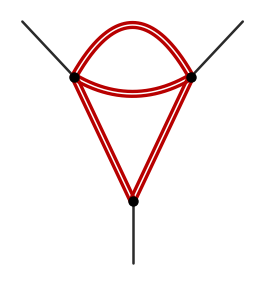
New transcendentala number satisfying no polynomial equation with integer coefficients — $\pi$ and $e$ are the classic examples numbers, given definitions instead of digits. The two-loop ice-cream cone — a triangle "cone" with a bubble "scoop" on its top edge — shows the arithmetic stakes of the portfolio most clearly. Its answer reduces to a single boundary number, and that number is a genuinely new period: for the equal-mass cone it lives on the very same elliptic curve as the sunrise and yet a lattice search shows it satisfies no relation in any classical ring of constants at the heights searched; for the cone with generic distinct masses the curve is non-modular and the boundary has no named home in any ring tested. Both constants are derived by two independent routes that agree — analytic matching at a special point of the integral's differential equation, and direct evaluation of a written-out convergent integral — and the closed forms pass their independent checks at 284, 110, and 133 digits across the family's three rows. The same closed form settles a question inherited from the S-matrix program of the 1960s: the strict hierarchical principle of Landshoff, Olive and Polkinghorne — the rule that a more complicated diagram should not suddenly switch on singularities none of its sub-diagrams predicts — for which Hannesdóttir, McLeod, Schwartz and Vergu had identified the ice-cream cone as the flagship counterexample by geometric argument. The bootstrapped formula exhibits the violation as an explicit nonzero number (the ice-cream-cone page; the fully worked example is Section 3 of the geometry paper).
Four new light-by-light integrals, one of them predicted before it could be checked. Light-by-light scattering — photons scattering off photons through a loop of massive charged particles — contributes at three loops a family of integrals that had no closed form in the literature; all four are closed here: the box with a sunrise inserted on one rung, the box with a kite inserted, and the kite insertion's two QED parent graphs. The first of these was written out in full, its boundary constant named in the curve's own ring as $2\,\mathrm{Cl}_2(\pi/3)$, before any independent value for the integral existed; the comparison was then run once, and the prediction matched at 71 and 69 digits at two fresh kinematic points. The other members close through dispersion relations — reconstructing the integral from its behavior across production thresholds — with every ingredient explicit, and agree with fully independent evaluations at 37–43 digits (the light-by-light page).
Fifteen of the thirty rows are new in this strong sense — no prior cross-validated computation found in the literature, several of them named as open problems by the papers that came before. Their tiles are in the grid at the top of this page; each links to a deep page with the full closed form and its evaluator.
A prediction, tested. One number in the crossed light-by-light box row was a prediction outright: no independent computation existed at $s=-7$, and the closed form gave the top integral's stripped on-curve value there as $-10.41519682\ldots$, written to 122 digits in July. An independent computation at $s=-7$ has since been made: an AMFlow run at that point agrees with the recorded value on 72 digits — the run's own depth, not the prediction's — and the prediction stands as the seventh point checked against a value that entered no fit.
The fifteen blind reproductions. Trust in the fifteen new results rests on known ground: fifteen rows of the portfolio recompute known results — several among the hardest in the literature — with the published values withheld from every derivation step, entering only the final comparison. Smirnov's 1999 closed form for the massless double box comes back coefficient by coefficient; the outer-mass double box of Caron-Huot and Henn returns as a single basis vector whose one rational coefficient must come out exactly 1, and does; the sunrise family — the door into elliptic Feynman integrals — matches at 149–159 digits across its mass configurations; the equal-mass kite of Adams and collaborators and the $gg\to H$ elliptic masters pass as well; the central-mass double box of Schwanemann and Weinzierl, re-derived through weight four without their result as input, agrees with their published program at two Euclidean points. At the top of the ladder, the three-loop banana of Pögel, Wang and Weinzierl passes at the K3 rung, and the four-loop Calabi–Yau banana is delivered as an explicit series solution with its complete boundary derived rather than fitted, matching an independent computation by Bessel moments at 116 digits, the reference method's own cap. An agreement of 150 digits between two independently computed numbers is a coincidence no wrong function survives. The fifteen are tiled in the grid at the top of this page.
The table as a whole. The portfolio's table has thirty rows — the next-order terms of the sunrise and the ice-cream cone in the $\varepsilon$-expansion counted as rows of their own — and not one of them is numerical-only. Every row ends in an explicit symbolic formula together with a standalone evaluator that recomputes it at any kinematic point and any precision with no loop-integral software running anywhere, and every row agrees to thirty digits or more with independent values withheld from its derivation. Twenty-four of the thirty were pinned by geometry, analytic constraints, and integer-relation fits; six went through the integration leg under the same acceptance standard. Two caveats are part of the record: five of the polylogarithmic rows were checked against analytic reference results rather than independent numerics, because the auxiliary-mass method that supplies the independent values everywhere else has no anchor for fully massless integrals; and one further row, the physical three-loop light-by-light parent, is listed in the paper but not counted, its blind cross-validation pending. Across the closed set, one thing varies: the arithmetic of the single boundary constant each row reduces to. Where the geometry supplies a named ring, the boundary is a classical constant — $\zeta_3$ for the K3 banana, a Chowla–Selberg period in its deeper layers, Catalan's constant on the $\Gamma_0(4)$ spine of $gg\to Z\gamma$. Where it does not, the boundary is a genuinely new transcendental, delivered as a written-out convergent integral and proven by theorem to carry no classical name. Beyond the computations themselves, each answer comes with a proof of what kind of number it is.
Results: Feynman geometry
The geometry paper’s results concern the geometry underneath the integrals rather than the integrals themselves: new structure at the physical thresholds, and proofs that some hoped-for answers do not exist.
Discoveries about the geometry itself. The setting is the banana tower: the sunrise generalizes to the $L$-loop banana graphs, whose underlying geometry climbs one rung per loop — a torus at two loops, a K3 surface at three, a Calabi–Yau threefold at four. A bootstrap that starts from the physics is forced to understand these families at their normal thresholds, the kinematic points where production of the internal particles switches on, and the new structure sits there. At its threshold the sunrise torus degenerates through an additive fiber of Type III in the Kodaira classification — the standard taxonomy of the ways an elliptic surface can degenerate — with finite local monodromy of order four (monodromy describes how solutions transform when carried around a singular point). This is the first non-semistable degeneration identified for a Feynman elliptic surface, verified four independent ways. An earlier reading placed the same fiber inside a five-propagator integral, the threshold kite; that family has its massless line on the rung, its cuts are genus zero, and it carries no elliptic curve, so the threshold sunrise remains the one Type III carrier. The pattern climbs the tower with period two — monodromy orders 4, 2, 4, 2 — with one caveat: no five-loop graph realizing the top rung as a genuine threshold has been exhibited, so that rung is conjectural. The threshold constants themselves close in classical rings: an exact projector built from the threshold monodromy delivers the K3 connection coefficient in closed form, $c_{3/2} = -\sqrt{3}/(36\pi)$, verified to 195 digits with an independent check to 80, and at the Calabi–Yau rung the conjugate pair $c_{5/4}, c_{7/4}$ closes in the lemniscatic $\Gamma(\tfrac14)$ ring — the ring the tower's order-four rungs share, beginning with the threshold sunrise, and here at the first Calabi–Yau dimension where it enters (the geometry paper).

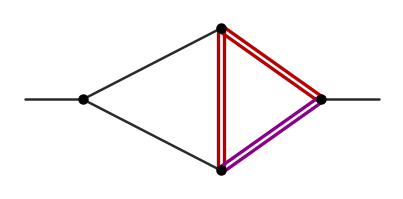
Figure 6. The banana tower’s thresholds alternate with period two, and their constants close in classical rings. Each loop climbs one rung of geometry — torus, K3 surface, Calabi–Yau threefold — with the graphs drawn in the site’s convention: double red lines are unit-mass propagators, and the violet line is the heavy propagator whose mass equals the sum of the rest, the coalescence that puts the graph at its threshold (the equal-mass sunrise instead sits at its normal threshold in momentum, $p^2=9m^2$). At the threshold the local monodromy (how solutions transform when carried around the singular point) alternates 4, 2, 4, 2 up the tower, verified by exact Picard–Fuchs indicial polynomials at all four rungs; the five-loop rung is stated by analogy, since no five-loop graph realizing it as a genuine threshold has been exhibited. The new threshold constants: $c_{3/2}=-\sqrt{3}/(36\pi)$ at the K3 rung, verified to 195 digits, and the conjugate pair $c_{5/4},c_{7/4}$ in the lemniscatic $\Gamma(\tfrac14)$ ring at the Calabi–Yau rung, verified to 197 digits — the lemniscatic ring, which the tower’s order-four rungs share from the threshold sunrise up, at its first Calabi–Yau rung. (Chart drawn for this page from the geometry paper’s data.)
Failed fits promoted to theorems. A fit that fails is a statement about the function space, and three such statements are proved.
- For the $gg\to Z\gamma$ masters, a blind fit of the boundary is provably impossible: the attempt plateaus at 1.43 digits of agreement while a positive control in the same setup reaches 78, and the obstruction — mixing between a period and its partner Eichler integral — is structural, not numerical. This is why the boundary is delivered as a named modular integral rather than a fitted number.
- For the three-loop crossed light-by-light box, a generalized-polylogarithm closed form for the top integral provably does not exist in any basis: the function is an iterated integral over a K3 period, a genuinely higher class of function. A companion system-level theorem — no finite-depth iterated-integral form exists in the family's raw frame — comes with a machine-checkable certificate, an exact witness file plus a short standalone checker any reader can run (the crossed-box page).
- The banana tower cannot produce the hoped-for new kind of number. A weight-three period without complex multiplication — an arithmetic symmetry that special elliptic curves carry — cannot arise from this family: the candidate K3's transcendental part factorizes into two copies of the sunrise curve, which carries complex multiplication by $\mathbb{Q}(\sqrt{-15})$, and Livné's theorem closes the remaining escape route. In the geometry paper's words, more computing power yields more digits of the wrong kind of number.
Row by row: the thirty integrals
The thirty counted rows, numbered as in the portfolio paper’s table; each entry says what the integral is, what was new, and links to its deep page with the diagram, the closed form, the boundary arithmetic, and the evaluator.
- outer-mass double box — polylogarithmic
The planar two-loop double box of Caron-Huot and Henn, with all six perimeter propagators carrying a common mass and massless external legs — a calibration row whose answer, after the leading singularity is stripped, is a single weight-four symbol vector. The bootstrap recovers the published symbol exactly (one rational coefficient, equal to one) and the closed form matches fresh AMFlow values at four points that entered no fit to at least 39 digits. → the page - massless double box — polylogarithmic
The fully massless planar double box — Smirnov's 1999 closed form, the simplest genuinely two-loop two-scale massless integral — run as the calibration anchor. The regression reproduces the harmonic-polylogarithm tower in t/s coefficient by coefficient against the analytic oracle (no massless vacuum boundary exists for AMFlow, so this is an oracle-target row). → the page - three-loop ladder — polylogarithmic
The three-loop planar massless ladder, the L=3 member of the Usyukina–Davydychev conformal-ladder family, whose finite part is a single tower of classical polylogarithms in one ratio. The lattice fit recovers every rational coefficient exactly, checked against the never-fit UD/Isaev analytic oracle values at roughly 450 digits. → the page - one-loop pentagon — polylogarithmic
The one-loop massless pentagon with five on-shell legs — the widest-alphabet polylog stress test in the portfolio, with 16 letters already at weight two. The finite part closes exactly as the five one-mass boxes with unit coefficients (the Bern-Dixon-Kosower form), the parity-odd Gram-determinant letter predicted absent through weight two, checked to 60 digits against the never-fit analytic oracle. → the page - Sudakov vertex — polylogarithmic
The two-loop massless Sudakov ladder: six massless lines, one off-shell leg, a single scale — the narrowest alphabet in the portfolio, so all the difficulty migrates into transcendental weight. Closed in exact form from the family's own reduction onto three Gamma-function masters: a pure zeta-value tower of uniform weight, order by order, agreeing with an independent numerical evaluation to at least 78 digits at every order. Restated 2026-09-03 after an erratum: the closed form previously reported here described a seven-line object that is not a graph. → the page - equal-mass sunrise — elliptic
The two-loop equal-mass sunrise at eps^0 — the simplest Feynman integral whose maximal cut is an elliptic curve, on the classical Gamma_1(6) geometry — run as the first elliptic calibration. The pipeline reproduces the Adams-Weinzierl closed form with every constant named (the boundary is (3/2)sqrt(3) L(chi_-3, 2), the function the Eichler integral of the weight-three Gamma_1(6) newform), passing the 30-digit never-fit gate against AMFlow with the boundary constant matched to 70 digits. → the page - sunrise (1,1,2) — elliptic
The two-loop sunrise with mass-squared assignments (1,1,2) at eps^0, where the unequal masses replace the equal-mass thresholds with an algebraic threshold letter and Abel-Jacobi marked points on the curve. Closed as an explicit Kronecker-eMPL form with PSLQ-exact rational coefficients [-1, -1/3, 8/3], checked against never-fit AMFlow values at 159 digits — the function space is classical; the new result is the cross-validated closure through one pipeline with every constant identified. → the page - sunrise (1,2,3) — elliptic
The two-loop sunrise with mass-squared assignments (1,2,3) at eps^0, the generic member of the family with all three marked points on the elliptic curve distinct. It closes by the same uniform per-puncture Kronecker-eMPL formula as the (1,1,2) case, checked against never-fit AMFlow values at 159 digits. → the page - sunrise (1,1,4) — elliptic
The two-loop sunrise with mass-squared assignments (1,1,4) — an unequal-mass configuration where the elliptic curve leaves the equal-mass Gamma_1(6) point. Closed in explicit Kronecker-eMPL form with PSLQ-exact rational coefficients by the same per-puncture formula that covers the whole mass family, validated against never-fit AMFlow values to 149 digits. → the page - sunrise at $\varepsilon^1$ — elliptic
The eps^1 correction to the two-loop sunrise, carried across all three unequal mass-squared assignments (1,1,2), (1,2,3), (1,1,4) and counted as a row of its own. It closes in a zero-parameter form — the weight-two eps^0 master plus a depth-three Kronecker-eMPL polynomial, with the one mixing constant an exact analytic frame factor rather than a fit — checked against nine independent AMFlow values, none of them held out, to 158–308 digits, the floor at each point being its reference's own goal. → the page - equal-mass kite — elliptic
The equal-mass kite: the two-loop self-energy graph obtained by hanging a massless rung across the equal-mass sunrise, whose Gamma_1(6) elliptic curve it inherits. A known integral (Adams et al.) rerun as a calibration: the five-term modular eMPL word list is re-derived blind through the pipeline, every coefficient a PSLQ-clean rational times a known constant (the only non-rational is the Clausen value Cl_2(2pi/3)), passing the >=30-digit never-fit gate. → the page - $gg\to H$ elliptic masters — elliptic
The elliptic master integrals of the two-loop mixed QCD–electroweak gg -> H amplitude, which live on the (m_t, m_t, M) two-mass sunrise curve with M an electroweak scale. A known family run as calibration: the two elliptic functions G_1, G_2 re-evaluated from the source paper's own one-fold period-integral definitions and checked to 48 digits against a never-fit auxiliary-mass-flow evaluation through the source's canonical rotation; the eMPL form of the masters, which the source paper left to future work, is not attempted. → the page - three-loop banana — K3 surface
The three-loop equal-mass banana at ε⁰: a two-point integral with four equal-mass propagators whose maximal cut is a K3 surface, the symmetric square of the sunrise elliptic curve. A calibration of the pipeline on the known Pögel–Wang–Weinzierl integral, delivered as the explicit two-term closed form m₁[ε⁰] = 7ζ₃ ϖ₀(t) − Part_reg(t) over a certified six-letter Γ₁(6) ε-form connection, matching the never-fit AMFlow oracle to at least 110 digits at eighteen points. → the page - four-loop banana — Calabi–Yau
The four-loop equal-mass banana at ε⁰, a two-point integral with five equal-mass propagators whose maximal cut is the holomorphic period of the one-parameter Hulek–Verrill Calabi–Yau threefold (operator AESZ #34). A known integral delivered as an explicit log-Frobenius solution of all five masters at the maximal-unipotent point, with the complete boundary derived in the ζ-ring (a rank-25 linear system with a unique solution, zero free constants) and agreement with an independent live Bessel-moment oracle at 116 digits, the oracle's own cap. → the page - central-mass double box — polylogarithmic
An independent computation of a known result: the two-loop planar double box with four massless legs and a single mass on the central rung (the γ-Z-γ ladder of NNLO electroweak Møller and Bhabha scattering), three scales, weight four, over a seven-letter rational alphabet. Closed in explicit two-variable form through weight four with only classical constants (zeta_2, zeta_3, zeta_4 and logarithms), agreeing with topology C of Schwanemann and Weinzierl (arXiv:2412.07522) and checked against never-fit AMFlow values at 109-112 digits on twenty points. → the page - non-planar hexa-box — polylogarithmic
The lightest crossing of the two-loop five-point non-planar hexa-box — equal-mass off-shell legs at the non-adjacent positions p1^2 = p3^2 = m^2, a 98-master family in the class bottlenecking NNLO diboson-plus-jet (VV'+jet) predictions. All 13 genuinely new master representatives are closed, the three top-sector masters as exact variation-of-parameters layered iterated-integral forms gated by the standalone evaluator at 66-68 digits at points that entered no fit, with all 447 tagged boundary constants recomputed at runtime from symbolic Gamma-form seeds at 81-100-digit two-precision agreement. → the page - unequal-mass kite — elliptic
The kite with unequal internal masses, where the sunrise sub-curve becomes genuinely non-modular and the value-fittability criterion proves in advance that a holomorphic weight-graded fit must fail. Closed instead by differential-equation transport seeded analytically at s=0 from the closed two-loop vacuum ring — every boundary constant classical (gamma_E, zeta_2, ln 2, Catalan), with the boundary period identified as a period of a specific conductor-128 curve carrying no shorter classical name — and AMFlow used only for the never-fit check, passed at 125–130 digits. → the page - equal-mass ice-cream cone — elliptic
The equal-mass ice-cream cone, a two-loop three-point graph (a massive triangle 'cone' with a bubble 'scoop' on its top edge) whose eps^0 top master is a weight-three elliptic function reducing to a single boundary constant. That constant is a genuinely new relative-cohomology period living on the same Gamma_1(6) curve as the sunrise yet proven to lie outside the sunrise's Eichler ring; it is now derived by two independent routes — analytic matching at the infinity cusp and a written-out convergent period integral evaluated to 284 digits — with AMFlow serving only as the never-fit gate. → the page - generic-mass ice-cream cone — elliptic
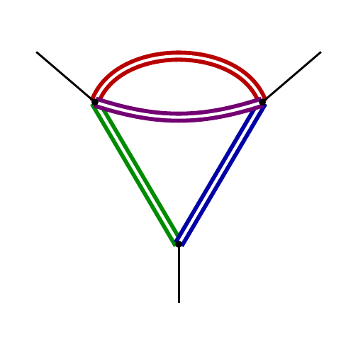
The ice-cream cone at generic distinct internal masses, whose (1,3,5) scoop sunrise curve is non-CM and non-modular: its boundary is a weight-three period with no named home in any classical ring tested. The boundary is derived analytically (including the exact cusp datum tau_0 = ln 15 · ln(1+sqrt 2)/sqrt 2) and materialized as an explicit convergent period integral, with the never-fit AMFlow gate passed at 110 digits, the full length of the reference values. → the page - ice-cream cone at $\varepsilon^1$ — elliptic
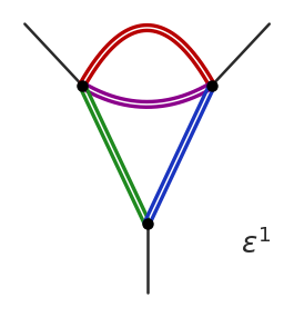
The eps^1 (weight-four) order of the ice-cream cone, equal-mass and generic, written out as an 88-term word list with exact Q(sqrt 5) residues. Its boundary constants close in the golden dilog ring (Tri_0, J, K), and the one remaining constant is a genuinely new weight-four transcendental — a relative-completion Eichler integral on X_1(6) with non-cusp marked points — derived rather than fitted and gated against never-fit AMFlow values at 133 digits. → the page - $gg\to Z\gamma$ at exact $m_t$ — elliptic
The pair of elliptic master integrals governing gg -> Z gamma with the exact top-quark-mass dependence, a configuration with no closed elliptic masters found in the literature. The closure carries zero AMFlow-derived constants — the corner masters close in 3F2/2F1 form, all 25 cusp conditions are proven analytic, the t-dependent tail is an exact polynomial, and the elliptic boundary is the named cusp-regularized Eichler integral on Gamma_0(4) — with never-fit AMFlow agreement at 126–139 digits. → the page - massless-rung kite, four masses — polylogarithmic
A two-loop kite with squared masses (1,4,9,2,0): two massive lines on each rim and a massless rung joining the internal vertices, so both three-line cuts pass through the massless line, their maximal cuts have genus zero, and no elliptic curve appears; the alphabet has seven letters, two of them quadratic, over four square roots. Genuinely new (no prior computation at these masses found): a 22-master transport from the analytic p^2=0 vacuum seed, the homogeneous constants fixed by boundedness at p^2=0, checked against never-fit AMFlow values at 81–110 digits on seven points, and reproduced at a second configuration, (1,4,9,3,0), at 98 digits or more on two points whose transported values were on record before the comparison. → the page - light-by-light (sunrise) — elliptic
A genuinely new three-loop light-by-light topology: the one-loop massive box (four on-shell photons, mass-m internal edges) with the two-loop equal-mass sunrise self-energy inserted on one rung, so the only elliptic curve in the problem is the inherited Γ₁(6) sunrise curve. The closed form, with its ε⁰ boundary constant named in the curve's own ring as 2 Cl₂(π/3) = (3√3/2) L(χ₋₃,2), was recorded in full as a prediction before any oracle output existed and then passed an independent AMFlow gate at 71 and 69 digits at two fresh points that entered no fit. → the page - light-by-light (kite) — elliptic
The one-loop massive light-by-light box with one rung replaced by the two-loop equal-mass kite self-energy, closed through a dispersion relation in which every ingredient is explicit: the spectral density is ρ(w) = −(π/w)[2 ln(w−1) ln w + 3 Li₂(1−w)] below the three-massive threshold plus a single one-fold over the Γ₁(6) sunrise cut above it, and the threshold constant A₁ = −2π is a theorem of the closed form rather than an input. The assembled integral agrees with a fully independent direct AMFlow evaluation to 43 digits. → the page - light-by-light (QED parent) — elliptic
The QED parent of the light-by-light kite insertion: the ten-propagator graph with two electron stubs flanking the kite self-energy (every vertex a genuine electron–photon vertex), of which the pinched graph is the limit. Both parent members close with the same closed-form kite spectral density through partial-fraction stub kernels, gated at 39 digits against an independent AMFlow oracle never used in the construction. → the page - light-by-light ($N_f^2$) — elliptic
The N_f² member of the light-by-light family, the box with a vacuum-polarization-type self-energy insertion, delivered by the same dispersive construction with the density symbolic exactly in d: an exact two-body cut in Γ-functions plus an exact-in-d one-fold over the Γ₁(6) sunrise cut for the three-body channel, its normalization derived rather than fit and no AMFlow input anywhere in the construction. The fixed-ε values agree with independent three-loop AMFlow evaluations never used in the computation to 76 digits or more at four Euclidean points, against higher-order grids (37–38 against the standard-order grids bundled with the script). → the page - $q\bar q\to W^+W^-$ non-planar — elliptic
The nonplanar T₄ branch of two-loop q q̄ → W⁺W⁻ with exact top-quark mass, the branch the planar literature computation explicitly left to future work; to our knowledge its first computation. On a one-dimensional kinematic line the 76 masters (23 genuinely new, including a new z₅-fibered elliptic curve in sector 481) are solved in explicit symbolic form — GPL words over the line alphabet, layered variation-of-parameters containers, and a rank-six thimble basis for the elliptic block — with all 79 basis rows gated at two fresh never-fit points (worst 37 digits at 40-digit working precision, rising to 57 at 60) and every boundary constant AMFlow-free by definition. → the page - threshold banana (K3) — K3 surface
The three-loop banana with masses (1,1,1,9), sitting at the mass coalescence where the K3 acquires order-2 non-unipotent monodromy. An exact spectral projector onto the −1 eigenspace of the threshold monodromy annihilates the unipotent log-tower algebraically and delivers the connection coefficient c₃∕₂ = −√3/(36π) in closed form, PSLQ-identified and verified to 195 digits, with an independent GKZ oracle agreeing to 80 digits. → the page - threshold banana (CY) — Calabi–Yau
The four-loop banana with masses (1,1,1,1,16), where the Calabi–Yau threefold acquires order-4 non-unipotent monodromy at the coalescence threshold. The spectral projector lifts to order four and closes the conjugate coefficient pair c₅∕₄, c₇∕₄ in the lemniscatic Γ(1/4) ring, Arb-ball-certified to 197 digits; the closed forms and the indicial argument that forces Γ(1/4) are in the geometry companion. → the page - crossed light-by-light box — polylog + K3
The three-loop crossed light-by-light box: a massive fermion loop around the four box-perimeter lines with two crossed massless photon diagonals and four on-shell external photons (the K₄ topology, sector 938 of the LBL3Q parent), a mixed family whose polylogarithmic top sector sits over a K3 banana sub-sector. The ε⁰ top master is closed as an exact word list over 13 quadrature letters — with a generalized-polylogarithm form proven nonexistent, since the function is an iterated-K3 integral — passing a never-fit gate against a reserved oracle at 72 digits (49 at the two-precision pair); the assembled evaluator is served on the page as a standalone script, and off the curve the leak term of the top block is fitted exactly on 37 rays with two further rays held out and reproduced entry for entry (790 of the 828 entries per node; no off-curve evaluator of the amplitude is claimed). → the page
Tools used
Every package below has its own page in the program's tool registry (the full index), where its mechanism, validation record, and limits are documented; the registry, not this list, is the citable record. The papers describe roughly a hundred program-built tools alongside the public engines they adopt; the registry consolidates them into packages, and the packages below are the ones the three papers used, in roughly the order the pipeline reaches for them — reduction, then singularities and geometry, then differential equations and transport, then evaluators, oracles, and the closure step that turns high-precision digits into exact statements. An oracle here is an engine that supplies high-precision numerical values of an integral: the raw data the fits consume and, kept strictly separate, the independent values a finished result must reproduce. Packages marked adopted are community software the harness consumes or ports; everything else was written inside the program because no public equivalent existed.
- Kira (adopted) — the integration-by-parts reduction engine of Maierhöfer, Usovitsch, and Uwer, later Klappert, Lange, Maierhöfer, and Usovitsch, with its finite-field library FireFly: the linear-algebra stage that rewrites the thousands of integrals a diagram family generates in terms of a few master integrals, the basis every later stage works over. The program runs it hardened: rebuilt against a fragmentation-resistant memory allocator after crashes with memory still free in aggregate, a 128-bit build for a job that overflowed the released version's 64-bit integer packing, parallel identity generation checked entry for entry against the serial reference, and chunked system encoding that completed a job repeated attempts had failed to finish. Every fix is preserved in an open repository.
- Blade (adopted, ported) — a reduction engine with a different cost model, implementing the block-triangular form of Guan, Liu, and Ma: one up-front search finds an equivalent system with far fewer equations, after which the reduction re-evaluates cheaply at every new kinematic point — precisely the access pattern of a method that samples the same family at many points. The toolkit's port runs it with no Mathematica kernel.
- Seedling — measured-support seeding for the reduction engines: before a large reduction launches, it reads off which seed identities the targets actually touch, pins the job to exactly that support, and predicts the memory cost from first principles. On its first production target it turned a staging run that had died of memory exhaustion into a routine job whose peak matched the prediction made before launch.
- Single-sector reduction (a routine written for the three-loop light-by-light calculation, not a released package) — one sector's differential equation without reducing the whole family (a sector is a sub-family of integrals sharing one set of propagators). It generates only the identities that sector needs and replays recorded eliminations across kinematic points, matched exactly against full reduction tables wherever both exist.
- Trust — the reduction-verification package, built on the observation that the folklore check — reduce twice, compare — cannot catch an error made the same way twice. Its independent reducer takes a second mathematical route (syzygy towers rather than Laporta elimination) and was run against production reduction tables, matching them on every comparable target.
- Winnow — the elimination step of Laporta reduction as a callable library, with a certificate attached to every row it returns. Its per-row multiplier certificates verify identities from any solver, and the package's canonical regression case is a reduction table that was measured, plausible, and wrong — the failure class only a per-row certificate catches.
- Seedling’s family preflight (folded from Family Audit) — pre-flight identity checks that settle what an integral family actually is before anything expensive runs on it. Its identity check matches the two Symanzik polynomials — the graph polynomials that define the integral — through an exact affine dictionary, proving two transcriptions are the same integral or that no identification exists; it exposed a transcription that silently defined a 98-master family where the corrected family has 76, and it is now a mandatory preliminary whenever a family is imported from the literature. A companion symmetry finder catches discrete automorphisms that Kira's own search does not look for.
- Numkin — the fix-one-scale instrument, and the method paper's chosen specimen of how the toolkit grows: it began as a hardwired workaround inside one stuck light-by-light computation and was generalized into a family-agnostic package. The move it packages is fixing one scale at a time — substitute an exact rational value for one kinematic invariant directly in the already-generated system files, run cheap lower-dimensional solves, and reconstruct the fixed variable exactly by interpolation, accepting an entry only when the reconstruction reproduces points it never consumed. One control is on record: offered too few points to determine a reconstruction, it excludes the entry rather than fabricate it.
- Formglue and FORM (FORM adopted) — FORM is the veteran symbolic-algebra engine for the enormous intermediate expressions of loop calculations; Formglue is the harness's routing and input/output around it, including a zeta-value oracle mode whose output is checked against independent references at essentially every digit of its working precision.
- PLD and SOFIA (adopted) — two engines from computational algebraic geometry that read a Feynman graph and return the places its integral can become singular: the Landau locus, governed by equations as old as the analytic S-matrix but push-button only since Mizera and Telen made the problem computational algebra in 2021. PLD.jl, by Fevola, Mizera, and Telen, is consumed as released; SOFIA, by Correia, Giroux, and Mizera, published in Mathematica, was ported to Julia so the alphabet search runs with no Wolfram kernel — a port whose defects had to be found and fixed before the published alphabet could be recovered, each fix now part of the released code.
- Landau Alphabet — the toolkit's implementation of the Landau bootstrap of Hannesdóttir, McLeod, Schwartz, and Vergu, the method that constrains an integral from its Landau locus and the geometry of its maximal cut (the integral with every propagator put on shell, which isolates a sector's intrinsic geometry). Its engine, LandauBootstrap, is a Julia rewrite of the method's original Mathematica research code: it builds the space of candidate answers as words over the symbol alphabet and drives the constraint cascade. In the method paper's calibration on the outer-mass double box it reproduced the published constraint cascade exactly, then closed the remaining fit from a fraction of the published sample budget (the full episode is under Approach).
- Ansatzer — the residual-count predictor: before a single oracle point is spent, it estimates what the constraint cascade will leave. On one five-point sector it predicted a residual of 42 functions against the sector's 200, so the expensive sampling stage is sized rather than guessed.
- Leviathan — a third singular-locus engine, independent of PLD and SOFIA: it locates singularities as the kinematic points where the integrand's critical values collide, read through a drop in an Euler characteristic, and it serves as the completeness check on symbol alphabets before they are believed. It has one recorded candidate blind spot, on a single row of the portfolio.
- GeoTriage — the geometry router: it reads each sector's maximal-cut geometry from algebraic invariants before anything is computed — polylogarithmic, elliptic, K3, or Calabi–Yau, in ascending order of geometric complexity — and so decides which function family the answer can belong to. It drove the geometry paper's discovery that the sunrise threshold degeneration is non-modular, and its one-call classifier reproduces every known reference verdict it has been tested on.
- Dipstick — triage before commitment: it reads the order and rank of a sector's Picard–Fuchs operator — the differential operator the sector's periods satisfy, whose order separates elliptic from K3 from Calabi–Yau — stable across two independent prime computations, before any expensive stage has run. The sunrise returns order 2 and the three-loop banana order 3 with no reduction run at all.
- Maxcut — the maximal-cut kit, one package for everything the pipeline does at the level of the cut: classify its geometry sector by sector, rotate a raw reduction basis into the canonical basis the cut implies — the program's rule is to sample and fit only in that basis, where fitting weight by weight is meaningful — and run the sparse constraint cascades. Its cascade collapsed the crossed light-by-light box's weight-five chain from 3352 unknowns to 20 through four exact stages, where the dense computation would have been out of reach.
- SubTropica — a symbolic integrator for parametric representations: hyperlogarithms with tropical subtraction, sector by sector, no Wolfram anywhere. It is the direct-integration leg for rows whose answers can be integrated outright, and its first production use returned an exact zeta-valued answer; on the crossed light-by-light box this leg cannot start at all, and that row is solved by a different route.
- Coalescer — reads the exact coefficient of a fractional-power threshold branch directly off the differential operator's monodromy, with no integration performed. It was trusted only after reproducing the K3 threshold constant $-\sqrt{3}/(36\pi)$ as a positive control, and then delivered the Calabi–Yau threshold coefficient; the spectral projector at the heart of the geometry paper's threshold results is documented on its page.
- Counterweight — the $\varepsilon$-factorizer: it rewrites a family's differential-equation system into canonical $\varepsilon$-form — the basis, found by Henn in 2013, in which the equations solve order by order in the dimensional regulator $\varepsilon$ — one exact rational move at a time. On the hexa-box — a frontier five-point family of the portfolio — its orbit engine surveyed all 31 diagonal blocks and proved which of them admit no rational $\varepsilon$-form, the measurement that routed that row to the layered closure instead; on another sector it delivered a certified $\varepsilon$-form where the previous attempt had stopped.
- Wayfinder — for the sectors the triage proves cannot be value-fitted (value-fitting: recovering exact coefficients from high-precision values of the integral alone, without solving its differential equation), the equation itself must be built and solved. The sampler reconstructs the canonical differential equation from numerical samples of its connection, snaps every entry to an exact fraction, and its transport layer carries solutions from a known boundary to any kinematic point being checked.
- Vopclose — closes layered path differential equations by variation of parameters, layer by layer, in an exact function model closed under the operations the solution needs. It is the engine behind the hexa-box row: a 98-master path system solved into explicit closed form, with all 447 boundary constants recomputed at runtime rather than pasted in.
- Ratfit — numeric samples in, exact rational functions out: it rebuilds the exact rational data that reduction and transport need from high-precision samples. Its deeper fits repaired a sector where most entries had resisted reconstruction at the original sample depth.
- Annihilator — exact operator reconstruction from series: hand it the terms of a power series and it finds, in exact arithmetic, the differential operator that annihilates it. It is the data-route sibling of the direct Picard–Fuchs probes, validated by recovering a known order-five operator from series terms alone.
- Eichler — the elliptic and Calabi–Yau period library, written from scratch: periods, quasi-periods, Eichler integrals (the antiderivatives of modular forms that supply an elliptic answer's missing transcendentals), and modular numerics, with every public routine returning an enclosure — a value with a proved error bound — rather than bare floating point. It carries the L-value dictionaries that check boundary-constant identifications: after a constant on a conductor-four curve was asserted by analogy to be $L(\chi_{-3},2)$ when the curve in fact calls for the conductor-four Catalan constant, named constants are supplied only from the dictionary, each as an enclosure. Its members include the certified elliptic-polylogarithm evaluator and the cusp-regularized Eichler-integral transport that runs inside every elliptic closure — the machinery behind the $gg\to Z\gamma$ masters and the nonplanar branch of two-loop W-pair production.
- GPLEval — the polylogarithm evaluator behind the value-fits: harmonic and Goncharov polylogarithms — the iterated-integral generalizations of the logarithm in which most massless answers close — built letter by letter as power series with exact rational coefficients and summed numerically only at the end, so the numbers being fitted mean exactly the same thing as the basis functions in the fit.
- Frobenius — a p-adic route to boundary constants: numbers others obtain by integrating are reconstructed from the differential operator's behavior modulo primes. In the geometry results it rebuilds the modular L-value $L(f_3,2)$ from Hecke eigenvalues matched across ten primes, confirmed by a 55-digit integer-relation match to its Chowla–Selberg form — with no integral evaluated anywhere in the derivation.
- PentagonFunctions-cpp (adopted) — the community library of pentagon functions, the function class in which two-loop five-point amplitudes are expressed. In this program it checks the one-mass five-point rows at sixty-plus digits and, in the method paper's words, feeds nothing — a cross-check by design.
- GiNaC (adopted) — exact symbolic algebra and polylogarithm numerics in compiled C++. With the Walden–Weinzierl elliptic-polylogarithm evaluator built on it, it serves as the reference implementation against which the toolkit's own elliptic evaluators are compared.
- AMFlow (adopted, extended) — auxiliary mass flow, the method of Liu and Ma that evaluates any master integral to hundreds of digits by flowing an auxiliary mass, is the program's high-precision engine, in a double role the pipeline keeps strictly separated: some of its values are the samples the fits consume, and others are the independent values, withheld from every derivation step, that a result must reproduce before it is accepted. It runs through amflow-cpp, a Wolfram-free C++ port adopted under a fix-and-adopt audit — the algorithm sound, the precision plumbing and robustness patched — whose full test suite now passes, and every production number is accepted only on the digits where two runs at staggered precision goals agree; the port's own printed error estimates are never trusted. All patches live in an open repository.
- pySecDec (adopted) — sector decomposition, the direct numerical route that integrates the parametric representation head-on. It is kept precisely because it shares no machinery with Kira or auxiliary mass flow: the orthogonal second oracle, so that agreement between routes is evidence rather than echo.
- Nestor — the in-house quadraturenumerical integration — approximating an integral by weighted sums of sampled values oracle: high-precision numerical integration by nested tanh-sinh quadrature, reporting only the digits successive runs agree on. It is the quadrature layer under the program's stated digit counts wherever an integral is checked by direct integration.
- Arb and mpmath (adopted) — the arbitrary-precision substrates under everything: Arb's ball arithmetic — every number carried as a midpoint with a rigorous error radius — on the Julia/FLINT side, mpmath on the Python side. The certified claims in these papers ultimately rest on these two foundations.
- Baller — the program's certified ball-arithmetic instruments in one package: quadrature, transport, and enclosure tools built on the Arb substrate. It was added late in the program and backs the certified-enclosure legs of the newer evaluation routes, the Calabi–Yau banana oracle and several elliptic-row evaluators among them.
- Gatekeeper — the oracle bookkeeping layer: registries and rules that keep the independent oracles genuinely independent, so a value that fed a derivation can never double as the value that validates it. Its harness is released among the program's open repositories.
- PSLQ and LLL (adopted, disciplined) — integer-relation detection: the algorithms (PSLQ is due to Ferguson, Bailey, and Arno) that recognize a high-precision decimal as an exact combination of named constants, the step that turns digits into closed forms. The program runs them under a fixed discipline: bounded search heights, stability of every identification across two working precisions, and positive controls before any identification is believed. A search that finds nothing is reported as a quantified exclusion at its stated height, not as silence.
- Lockpick — lattice-based closure for the identifications plain PSLQ cannot reach: the LLL matrix machinery together with the curated ring of named constants the searches may draw on. The method paper's outer-mass double-box calibration closed through this route, the answer recovered as a single lattice vector rather than a term-by-term fit, the prediction carried at 64–66 digits of working precision.
- Per-row evaluators — where every solved integral ends up: a standalone script on the integral's own page (the tile's Downloads line) that evaluates its final form at any point and precision and checks itself against independent reference values.
- Single-problem instruments — beside the packages, the portfolio rows name a handful of narrower instruments written for one computation: the boxdilog exact one-loop-box kernel, the detrho transport (later superseded by a closed form), the etatail tail bound, and recon2var, svgalois, and rankscreen among them. These are documented where they are used, in the papers and the run records, rather than as standalone package pages.
Code
The released code is organized around the BootLoops standard stated under Approach: the explicit symbolic final form, the standalone evaluator, and reproduction of independent values withheld from the derivation. The portfolio paper states the question this answers: how does a reader check, with no trust in us and no loop-integral software at runtime, that this specific function is this specific integral?
Concretely, every row of the thirty-integral portfolio comes with its standalone evaluator — one Python script per row, eval_row07.py, eval_row14.py, and so on — that computes the row's closed form at any kinematic point and any requested precision, with no AMFlow, no Kira, and no integration-by-parts reduction anywhere at runtime; twenty-five of the scripts run from arbitrary-precision Python imports alone. Auxiliary-mass-flow numbers appear in a script only as reference values recorded in its header — digits the evaluation is compared against, never digits it computes from — and the papers print spot values at named kinematic points so a reader can re-check a row directly. The comparison is itself tested: on one of the kite rows, perturbing a single constant the evaluation depends on by one part in $10^{30}$ collapses the agreement from 125 digits to about 31, demonstrating that the comparison tests the computed value, not the pasted reference. Each row's exact data — conventions, alphabets, basis rotations, boundary constants — travels with it as ancillary files, and the geometry paper's theorem that the crossed light-by-light box admits no finite-depth function form in its raw frame is released as a machine-checkable certificate: exact witness data plus a short standalone checker script that recomputes the claimed structure from the witness and aborts if anything drifts.
The pipeline itself is public. It is built from community engines consumed as released and from the program's own ports and tools — in the method paper's words, there is no private black box anywhere on the critical path. The patched engines are open repositories, mattschwartz-sketch/amflow-cpp and mattschwartz-sketch/kira, maintained upstream-style with each defect documented at the point where it occurs and each repair available to be re-run and audited; the SOFIA.jl, Eichler.jl, LandauBootstrap, and oracle-harness ports are released alongside them. Production is deliberately Mathematica-free: at most one workstation license survives anywhere in the program, off the critical path, as a cross-validation oracle.
The documentation is the online tool registry, released with the program's code: one page per package, recording mechanism, validation, measured limits, and change history. The registry keeps its negative record at the same level of detail as its successes — withdrawn tools, refused inputs, and declared stubs are documented, not deleted — and the papers' own rule is that no measured number should be quoted without the configuration and caveats of its registry entry, which is the citable record.
Papers
Automated computation of Feynman integrals with BootLoops (PDF) — the method; Bootstrapping elliptic and Calabi–Yau Feynman integrals (PDF) — the geometry; Polylogarithmic, elliptic, and Calabi–Yau Feynman integrals from a hybrid bootstrap (PDF) — the portfolio.
References
| G. Passarino & M. Veltman (1979) | one-loop reduction — the loop problem solved as a class |
| K. G. Chetyrkin & F. V. Tkachov (1981); S. Laporta (2000) | integration-by-parts identities, and the algorithm that industrialized them |
| T. Gehrmann & E. Remiddi (2000); T. Gehrmann, J. M. Henn & N. A. Lo Presti (2016) | the differential-equation method at the two-loop frontier of its day |
| A. B. Goncharov, M. Spradlin, C. Vergu & A. Volovich (2010) | the symbol — polylogarithm algebra made a working tool |
| J. M. Henn (2013) | canonical differential equations — multiloop integration as linear algebra |
| A. Sabry (1962); S. Laporta & E. Remiddi (2005) | the sunrise: forty-three years from problem to first elliptic evaluation |
| S. Pögel, X. Wang & S. Weinzierl (2023) | the Calabi–Yau banana in $\varepsilon$-factorized form — the direct-computation landmark |
| X. Liu & Y.-Q. Ma (2022) | auxiliary mass flow — hundreds of digits at any kinematic point |
| S. Mizera & S. Telen (2021); C. Fevola, S. Mizera & S. Telen (2023); M. Correia, M. Giroux & S. Mizera (2025) | the Landau singular locus made push-button (PLD.jl, SOFIA) |
| S. Caron-Huot & J. M. Henn (2014) | the outer-mass double box — the calibration target |
| H. S. Hannesdóttir, A. J. McLeod, M. D. Schwartz & C. Vergu | the Landau bootstrap — one of the two parent methods |
| Barrera, Dersy, Husain, Schwartz & Zhang | analytic regression — the other parent; the elliptic case explicitly deferred |
| He, Zhang, Han, Jiang, Li & Wang | the planar W-pair branches with exact top mass — the nonplanar branch left to future work |
| Morales, Spiering, Wilhelm, Yang & Zhang | the symbol-level elliptic bootstrap that stopped short of the function level |
| V. A. Smirnov (1999) | the massless double box’s closed form — reproduced coefficient by coefficient |
| P. V. Landshoff, D. I. Olive & J. C. Polkinghorne (1966) | the hierarchical principle whose flagship violation is now an explicit number |
| H. R. P. Ferguson, D. H. Bailey & S. Arno (1999) | PSLQ — exact constants recognized inside long digit strings |
| This work: Automated computation of Feynman integrals with BootLoops (PDF); Bootstrapping elliptic and Calabi–Yau Feynman integrals (PDF); Polylogarithmic, elliptic, and Calabi–Yau Feynman integrals from a hybrid bootstrap (PDF) | the method, the geometry, and the thirty integrals |