Three-loop light-by-light
Four photons scattering off a closed electron loop, computed at three loops with the electron mass kept — five dressings of the one-loop box solved here, mapping which stay polylogarithmic, which turn elliptic, and which touch a K3 surface.
The content on this page was written by AI under human supervision.


The integrals
Light-by-light scattering is the process $\gamma\gamma\to\gamma\gamma$: four photons, all massless and on shell ($p_i^2=0$), interacting through closed loops of virtual electrons of mass $m$. This page covers the three-loop family with the electron mass kept. Every member is an integral of the form
$$I[\nu_1,\ldots,\nu_n](s,t;m^2)\;=\;\int d^dl_1\,d^dl_2\,d^dl_3\;\prod_{j=1}^{n}\frac{1}{D_j^{\nu_j}},\qquad d=4-2\varepsilon,$$
up to an overall normalisation convention, with propagators $D_j=q_j^2-m^2$ on electron lines and $D_j=q_j^2$ on internal photon lines, where each $q_j$ is the combination of the loop momenta $l_1,l_2,l_3$ and the external momenta flowing through line $j$. The Mandelstam invariantsthe Lorentz-invariant combinations of external momenta that a scattering amplitude can depend on are $s=(p_1+p_2)^2$ and $t=(p_2+p_3)^2$; the third pair-sum $u=(p_1+p_3)^2$ obeys $s+t+u=0$ because the photons are massless; and $m^2$, set to $1$, fixes the overall scale. Every family reduces to a finite basis of master integralsthe finite basis of independent integrals to which every integral of a family reduces by integration-by-parts identities, and all results on this page are at Euclidean kinematics ($s,t<0$), where the integrals are real.
Every three-loop one-fermion-loop diagram of the process is the one-loop electron box — four electron propagators forming a square, one external photon at each corner — with two extra internal photons attached at four points on the loop; the taxonomy is set by where those four points land on the box's four sides (its "rungs"). Adding a second closed fermion loop opens the $n_f$ classdiagrams with a vacuum-polarisation bubble on an internal photon — two closed electron loops instead of one. The geometry of each class's top sector decides how it can be solved:
| class | top-sector geometry | |
|---|---|---|
| (4,0,0,0) | two-particle-reducible self-energy on one rung | inherited Γ₁(6) elliptic |
| (2,0,2,0) crossed | crossed box | polylogarithmic top over the K3 banana at $u$ |
| $n_f$ | vacuum-polarisation bubble on the self-energy photon | inherited Γ₁(6) elliptic |
Five members are closed on this page — the (4,0,0,0) tower (the sunrise and kite dressings and the physical graph), the $n_f$ dressing, and the crossed box. The ten-line parent of the crossed box has not been computed; it is covered in its section below.
Why it matters
Classical electrodynamics is linear: two light beams pass through each other unchanged. QED predicts otherwise — four photons can scatter through a virtual electron loop — and the prediction has been seen. ATLAS and CMS have observed $\gamma\gamma\to\gamma\gamma$ directly in ultraperipheral Pb–Pb collisions; the same process is a clean search channel for axion-like particles. Pushing the QED prediction past two loops needs exactly these masters. At two loops the massive master integrals stay polylogarithmic (Ajjath–Chaubey–Shao); at three loops the massless-electron masters are known (Bargiela et al.), but with the electron mass kept we have found no master integral previously computed.
The five diagrams are also the cleanest demonstration that route follows geometry. Same process, same external state, same kinematics — and the attachment of the two extra loops forces entirely different mathematics:
- the two-particle-reducible dressings — a self-energy or vacuum-polarisation insertion on a rung — factorise exactly into one-dimensional dispersive integrals;
- the bare sunrise master carries the modular Γ₁(6) curve and closes through Eichler integrals;
- the crossed box hides a K3 surface under a polylogarithmic top sector: a closed form provably cannot be reached by fitting values against known constants, so the differential equation itself must be transported;
- the remaining two classes are geometrically mapped.
What was hard
Three-loop integrals with an exact internal mass have no ready-made function space: which sectors are polylogarithmic, which carry the Γ₁(6) elliptic curve, and which sit on the K3 surface of the three-loop banana had to be proven sector by sector from the graph polynomials — and that stratification, not the diagram's appearance, dictates every route below. For the two-particle-reducible members the three-loop system is never solved head-on: cutting the self-energy insertion factorises the integral exactly into a spectral density convolved with a one-loop kernel, and the real work is at the thresholds, where the closed-form turn-on of the density must be subtracted and re-added analytically for the convolution to converge. For the bare sunrise master the decisive step was the boundary anchor: a first seed from a Bessel-moment representation carried sub-topology contamination, and replacing it with the homogeneous Picard–Fuchs period — annihilated by the sunrise operator by construction, so there is nothing to contaminate — fixed the transport. The crossed box was the stress test: its finite master is provably beyond value-fitting, so its differential equation had to be completed and transported, and completing it exposed that one block of the stored connection was missing its sub-sector couplings — the absent entries were reconstructed exactly and matched against an independent symbolic reduction.
The results
The five closed members live in different function spaces, so each closed form is displayed in its own section: sunrise dressing, kite dressing, the physical graph, vacuum-polarisation dressing, crossed box.
---
Sunrise dressing (LBL3E)

The minimal elliptic three-loop master: replace one rung of the massive box with the equal-mass sunrisethe two-loop self-energy with three parallel massive lines between two vertices — the simplest Feynman diagram that produces an elliptic curve. Six lines, four vertices, all mass $m$. This is the deepest pinch of the family tower — the grandchild of the physical graph (shrink the physical graph's two electron stubs, then the kite's two photons, and you land here), and the place where the elliptic curve actually enters. The sunrise's Γ₁(6) curve is fibred over the box virtuality $w$ — the squared momentum flowing through the dressed rung of the box — with cusps at $w\in\{0,1,9,\infty\}$ and Kodaira fibresthe singular-fibre types of the elliptic fibration at the four cusps, in Kodaira's classification $(1,2,3,6)$. The reduction finds ten masters, of which seven carry the elliptic curve; the closed form below holds for all seven, with the homogeneous period computed two independent ways (a Frobenius power series of the Picard–Fuchs operator and a level-6 modular $q$-series).
The result
All ten masters of the sunrise-dressed box close at function level. The seven elliptic masters (sectors 15, 55a–e, 63) share one elliptic function — the uncut equal-mass sunrise on the dressed rung — and that function is one line:
$$\mathcal{I}_{\rm sun}(w)=\psi_1(w)\big[\mathcal{E}[f_3](\tau(w))+c_1\big]+c_2\,\psi_2(w),\qquad (c_1,c_2)=\big(B^{(0)},0\big),\qquad \psi_1=\tfrac{2\pi}{\sqrt3}\,\varpi_0.$$
Here $\psi_1(w),\psi_2(w)$ are the period pair of the $\Gamma_1(6)$ fibre curve at box virtuality $w$ — the two independent solutions of the equal-mass-sunrise Picard–Fuchs operator
$$L_{\rm sun}=t(t-1)(t-9)\,\frac{d^2}{dt^2}+(3t^2-20t+9)\,\frac{d}{dt}+(t-3),\qquad t=w/m^2,\qquad \varpi_0(0)=1,$$
with $\varpi_0$ the holomorphic Frobenius solution fixing the exact $2\pi/\sqrt3$ normalisation; $\tau(w)$ is the modular parameter of the fibre; $\mathcal{E}[f_3]$ is the Eichler integral of the weight-3 Eisenstein form $f_3$ on $\Gamma_1(6)$; and $c_1,c_2$ are the two boundary constants. The dressed sectors (55a–e, 63) do not take this period-times-Eichler form master by master: the dressing is a one-fold over a moving fibre, so no per-master constants exist as posed, and those sectors close through the dispersive one-fold assembly described below. The leading boundary constant is exactly
$$B^{(0)}=2\,\mathrm{Cl}_2(\pi/3),$$
with $\mathrm{Cl}_2$ the Clausen function; the sub-leading constants $B^{(1)}, B^{(2)}$ are given by the ${}_2F_1$ $\varepsilon$-derivative form, and a PSLQ search in the conductor-3 cusp ring alone finds no relation for either; both are identified once the log-sine integrals $\mathrm{Ls}_n^{(k)}(\theta)=-\int_0^\theta x^k\log^{n-1-k}\lvert 2\sin\tfrac{x}{2}\rvert\,dx$ are adjoined to that ring:
$$B^{(1)}=\tfrac{1}{6}\pi^3-2\log 3\,\mathrm{Cl}_2(\pi/3)+3\,\mathrm{Ls}_3(2\pi/3),\qquad B^{(2)}=-2\pi\zeta_3-\tfrac{1}{6}\pi^3\log 3+\log^2 3\,\mathrm{Cl}_2(\pi/3)+2\,\mathrm{Ls}_4(2\pi/3)-3\log 3\,\mathrm{Ls}_3(2\pi/3),$$
as integer relations of height at most 18, found on 120-digit values and again on a 320-digit re-evaluation of the ${}_2F_1$ form; $\mathrm{Ls}_3(2\pi/3)$ is the one new weight-three constant. The remaining three masters are polylogarithmic. The independent confirmation solves the uncut equal-mass sunrise — the elliptic content of these sectors — at box virtualities never used in the construction; the full box-dressed top master has since been evaluated directly as well — the box exactly as drawn in the figure at two points, 48 digits at each — and the box's top master is now assembled as a function of $(s,t)$ that agrees with independent evaluations at three Euclidean points — one of them predicted before its independent value was computed — to at least 45 digits at $\varepsilon^0$ (52–53 at the poles); that assembly is served as lbl3e-box-evaluate.py with its folder vendor_row27_box/, which rebuilds the top master at any Euclidean $(s,t)$ and checks the three recorded points, the third of them the one whose value was filed before its independent evaluation existed. A maximal-cut check of the dressed top sector is ill-posed — the cut pins $w=m^2$, a degenerate cusp fibre, and cannot see the elliptic modulus at all — which is why the independent confirmation runs on the uncut sunrise; the variation-of-parameters mechanics behind that shared elliptic content are validated to 116 digits. lbl3e-master-evaluate.py assembles the sector-15 master through ε² at runtime from the pieces above — both period routes, τ by two routes, the Eichler integral, the boundary tower — checks it against certified reference values, and checks the recorded independent AMFlow values against the locked prediction at $w=-7/3$ and $w=-4$, two points kept out of the construction; lbl3e-evaluate.py evaluates $\psi_1/\pi$ and $B^{(0)}$ alone. Downloads: lbl3e-expression.md · lbl3e-evaluate.py · lbl3e-master-evaluate.py · data: row27_data.json · row27_gate_amflow.json (the master evaluator reads both from its own directory) · lbl3e-box-evaluate.py (the box's top master as a function of $(s,t)$ with the three recorded points in vendor_row27_box/; the default run reproduces the first point at 32 digits in about three minutes, and --dps 48 reaches the recorded 45 digits in about ten; --route tanhsinh recomputes the same values by a second, independent integration route — a tanh-sinh quadrature of the dispersion-subtracted one-fold, its code shipped beside the script — and reproduces the served values to every printed digit at both precisions; --triangles checks the tower of generalised triangles that feeds the box's pole terms against two independent one-loop references shipped beside the script — AMFlow evaluations of the massless-insertion families and closed hypergeometric forms — coefficient by coefficient, agreeing to 31 digits at 32 working digits and 47 at 48, in about three and eleven minutes per point) · data: vendor_row27_eps1/ (the box's top master at order $\varepsilon^1$ at the first point: assembled at 32 and 48 working digits it agrees with an independent AMFlow evaluation to 30 and 46 digits, the two precisions agreeing with each other to 30; the folder holds the two assembly outputs, the AMFlow value with its configuration, the quadrature node sets and the assembler as run, and reproduce_eps1.py re-derives every digit count from those files in about a second — the hours-long assembly itself is not re-run) · MANIFEST.sha256 (every file of the bundle with its checksum)
---
Kite dressing (LBL3SE)

Replace the rung with the equal-mass kitethe two-loop rhombus-plus-diagonal self-energy in mass pattern (0,0,m,m,m); contains the sunrise as a sub-topology and inherits the same Γ₁(6) curve instead. Eight lines, six vertices, six massive electrons and two massless photons. This is the stripped master — the self-energy blob without its two flanking electron propagators, so it is not itself an all-$ee\gamma$ QED graph; the physical graph is the next section, whose pinch reproduces it exactly. Because the diagram falls into two pieces when the lines flanking the insertion are cut, the integral factorises exactly — the dispersive representation below is the closed form, not an approximation.
The result
The kite-dressed box is an exact one-fold over the internal mass of the dressed rung:
$$I(s,t,m^2)=\frac1\pi\int_{m^2}^\infty\!\rho(w)\,\mathrm{Box}_1(s,t;w)\,\mathrm{d}w,\qquad \rho(w)=-\,\mathrm{Im}\,J_{\rm top}(w+i0),$$
where $\mathrm{Box}_1(s,t;w)$ is the one-loop massive box with the dressed rung's squared mass set to $w$ — a closed dilogarithmic form — and $\rho$ is the kite's spectral density, the discontinuity of the kite top master $J_{\rm top}$. Below the three-particle threshold the density is the closed weight-2 form ($m^2=1$)
$$\rho(w)=-\frac{\pi}{w}\Big[2\ln(w-1)\ln w+3\,\mathrm{Li}_2(1-w)\Big],\qquad m^2\le w\le 9m^2,$$
and above it a $\Gamma_1(6)$ sunrise-period one-fold. The threshold turn-on coefficient $-2\pi$ is a theorem forced by regularity at $w=m^2$, not a fitted constant, and the large-$w$ tail is exact:
$$\rho(w)=\frac{4\pi\ln w+6\pi}{w^2}+\frac{8\pi\ln w+\tfrac{\pi}{2}}{w^3}+\cdots$$
Nothing is tabulated: the density is regenerated at any requested precision as a series solution of the exact rational kite differential system, from a single boundary seed itself derived from vacuum closed forms. The evaluator below also carries the density in the closed form written above: every run evaluates the dilogarithms below the three-particle threshold and the sunrise-cut one-fold above it at $w=5,\,12,\,100$ and checks them against independent AMFlow evaluations (to 65 digits or more) and against the series solution, which remains the dispersion integrand; its --sum-rule option checks the normalisation $\frac1\pi\int_{m^2}^\infty\rho\,\mathrm{d}w=6\zeta_3$ to 48 digits at the cutoff $W=10^{50}$, 62 with the leading tail restored. The same function is checked at a further Euclidean point, $(s,t,m^2)=(-1/2,-1,1)$, against an independent evaluation never used in the construction, to 59 digits; the evaluator below computes that point too (--point P1) and checks it against the recorded value. Downloads: lbl3se-expression.md · lbl3se-evaluate.py · kite_de_exact_parse.py (the exact parser of the kite connection the evaluator reads; plain Python, no computer-algebra system at runtime) · kite system · kite boundary vector · derived boundary seed from lbl3se-w5-seed.py · fast cache (optional; without it the script runs the full live computation; the cached values are certified to 43 digits by a two-precision comparison, and the script caps what it prints at that depth) · reserved point (the point the evaluator is checked at, now carrying two direct-solve reference strings of 290 digits; the point tier's bar, 55 digits, is what the evaluator itself reaches at that precision, and the recorded value's 59-digit agreement with the direct solve is printed beside it as the count of record) · MANIFEST.sha256 (every file of the bundle with its checksum). The evaluator reads every file from its own directory.
---
The physical graph (LBL3KP)

The actual QED amplitude piece — the top of the family tower shown above: keep the two electron stubs — short propagators $\ell^2-m^2$, with $\ell$ the loop momentum flowing through the stub — that flank the self-energy. Drawn physically, the kite is the crossed-photon self-energyemit γ₁, emit γ₂, absorb γ₁, absorb γ₂ on a straight fermion line — two interleaving photon arcs; topologically the same five-propagator kite as above. Ten lines, eight vertices, every vertex $ee\gamma$. The two stubs contribute a double pole at the threshold of the dispersive integral, which the subtracted kernel below removes exactly.
The result
The physical graph closes by the same dispersive factorisation, with the threshold pole of the doubled electron stub subtracted exactly:
$$I_{\rm KP}=\frac1\pi\int_{m^2}^\infty\!\rho(w)\,K_P(w)\,\mathrm{d}w,\qquad K_P(w)=\frac{K(w)-K(m^2)}{(w-m^2)^2}-\frac{K'(m^2)}{w-m^2},$$
where $\rho$ is the same kite spectral density as above, $K(w)=\mathrm{Box}_1(s,t;w)$ is the closed dilogarithmic one-loop box kernel, and $K'(m^2)$ is its derivative at the on-shell point. The single-stub and no-stub members of the same family use $K_1(w)=[K(w)-K(m^2)]/(w-m^2)$ and $K(w)$ with the same density, and the no-stub member reproduces the kite dressing above exactly. The identity behind $K_P$ is general: any self-energy-on-a-rung graph of this type reduces to divided differences of the bare-rung kernel against the unchanged sub-loop density. The one-fold representation lives in the insertion-mass variable, with all $(s,t)$ dependence in the kernel; a fully kinematic-space iterated-integral form was not built. The same further point, $(-1/2,-1,1)$, checks the physical graph and its single-stub member against an independent nine-propagator AMFlow $\varepsilon$-grid (twenty samples, extrapolated to $\varepsilon\to0$) to 50 digits each, and the same deeper grid at the reference point to 68 digits each — at the further point the 50 is the evaluator's own two-precision floor, the grid's bars (68 and 74 digits) sitting above it; at the reference point the evaluator agrees with the grid's extrapolation to 75 digits with its own two-precision floor at 102, so the count there is the grid's order-convergence bar, 68; the evaluator below computes the further point (--point P1, at 60 working digits) and checks both against the deeper grid's own extrapolated values, reaching 45–46 of their digits — the 50-digit counts are the record's run at 45 working digits, printed beside; the digits past 45 in the served script depend on its kernel fit's conditioning, a known limit named in the download. Downloads: lbl3kp-expression.md · lbl3kp-evaluate.py (every run also evaluates the closed-form density above — dilogarithms below $9m^2$, the sunrise-cut one-fold beyond — at $w=5,12,100$, checked against independent AMFlow values and the kite-system series that remains the dispersion integrand; --sum-rule checks $\tfrac1\pi\int\rho\,\mathrm{d}w=6\zeta_3$ to 48 digits at cutoff $W=10^{50}$) · kite_de_exact_parse.py (the exact parser of the kite connection the evaluator reads; plain Python, no computer-algebra system at runtime) · kite system · kite boundary vector · derived boundary seed from lbl3kp-w5-seed.py (a shim that runs the kite-dressing seed script above from a sibling lbl3se/ directory) · fast cache (optional). The evaluator reads every file from its own directory. · MANIFEST.sha256 (every file of the bundle with its checksum; the fast cache's values are certified to 38 digits by a two-precision comparison, and the script caps what it prints at that depth) · reference-point comparison (the objects behind the reference-point digit counts: the twenty-sample AMFlow grids, the evaluator's values there at 105 and 165 working digits with the records of how each was computed and assembled, the comparison script and its relative-digit re-reading — every digit count relative, the grid's absolute readings kept beside — and reproduce_p3.py, which re-runs the comparison in seconds)
---
Vacuum-polarisation dressing (LBL3VP)

The simplest two-fermion-loop member: dress the rung with the one-loop self-energy carrying a vacuum-polarisation bubblethe electron emits a photon, the photon splits into an $e^+e^-$ pair which recombines, the photon is reabsorbed. Textbook QED $\Sigma$ with the photon line replaced by the dressed propagator.. Ten lines, eight vertices, two closed fermion loops, and a double pole in $\varepsilon$ from the nested subdivergences. The two electron stubs flanking the insertion carry one and the same propagator, as do the two photon segments on either side of the bubble, so the ten lines are eight distinct propagators, two of them squared. This member closes as a full function of $\varepsilon$, poles included; $w'$ below is the squared invariant mass flowing across the self-energy cut.
The result
The vacuum-polarisation dressing closes as a full function of $\varepsilon$ — every factor a closed form or a one-fold over closed-form kernels, exact in $d$:
$$I_{\rm VP}(\varepsilon)=\frac1\pi\int_{m^2}^\infty\!\rho_{\rm VP}(w';\varepsilon)\,K_P(w';\varepsilon)\,\mathrm{d}w'.$$
On the two-body cut the density is elementary and exact in $d$ ($m^2=1$):
$$\frac{1}{\pi}\,\mathrm{Im}\,\Sigma_{\rm VP}(w';\varepsilon)=\frac{\Gamma(1+\varepsilon)\Gamma(1-\varepsilon)}{\varepsilon\,\Gamma(2-2\varepsilon)}\Big[{-}\tfrac{(1-2\varepsilon)(w'+1)}{w'-1}+\tfrac{\varepsilon(w'-1)}{6}\Big]\frac{(w'-1)^{-2\varepsilon}}{w'^{\,1-\varepsilon}}.$$
Above the three-body threshold $w'=9m^2$ the density is a $\Gamma_1(6)$ sunrise-period one-fold, also exact in $d$:
$$\rho_{3b}(w')=\pi\,c_1^2\,w'^{\,\varepsilon-1}\!\int_4^{(\sqrt{w'}-1)^2}\!\!dq\,(q-4)^{\frac12-\varepsilon}q^{-\frac52}\big[((\sqrt{w'}-1)^2-q)((\sqrt{w'}+1)^2-q)\big]^{\frac12-\varepsilon},\qquad c_1=\tfrac{\Gamma(1-\varepsilon)}{\Gamma(2-2\varepsilon)};$$
its branch points $\{0,4,(\sqrt{w'}\mp1)^2\}$ are the equal-mass-sunrise quartic, and at $\varepsilon=0$ it is the closed form of the elliptic remainder that refused every weight-2 polylogarithmic basis. The kernel $K_P$ is the same twice-subtracted box kernel as above, defined by an exact two-fold Feynman-parametric integral, exact in $\varepsilon$. The pole layers close analytically:
$$\Sigma_{\rm VP}^{(-2)}(w')=-\frac{1}{w'-1},\qquad \Sigma_{\rm VP}^{(-1)}(w')=-\frac{2\log(1-w')}{1-w'}-\frac{\log(1-w')}{w'}+\frac{2\gamma_E}{w'-1}.$$
Downloads: lbl3vp-expression.md · lbl3vp-evaluate.py · self-energy and box systems with their boundary data · comparison values · fast cache (optional) · MANIFEST.sha256 (every file of the bundle with its checksum). The evaluator reads every file from its own directory. The four Laurent coefficients at the reference point at full length — $c_{-2}$, $c_{-1}$, $c_0$ and $c_1 = 0.0397158224\ldots$ (two-precision stable to 46 digits; the dps-50 and dps-45 strings carry 56 and 51 decimal places) — are in laurent_coefficients_row33_20260909T043046Z.json beside the scripts; no script reads it. The $\varepsilon^0$ layer is served by a second script, lbl3vp-eps0-evaluate.py: it computes $c_0 = -0.1466053426\ldots$ as one finite subtracted integral — no $\varepsilon$ grid — with every truncation refined until its bound is met, and compares it with an independent reference value from the fixed-$\varepsilon$ route (32 digits at --dps 30, bar 20). It is a long run by design: 13 minutes at --dps 30 and 31 minutes at --dps 50 on a loaded 96-core server (measured); at the default --dps 110 the earlier step controller took 50,438 s = 14.0 h in all, 37,281 s of it in the kernel stage (controller-limited: 8,137 halved steps, each a recomputed series — the waste this release removes; the cured script's wall at --dps 110 is not measured), for the same 39.23 digits against the reference value as --dps 50, that value's own trust being 39 digits. The script saves its two transport stages as they complete and --resume continues an interrupted run from them. Its engine sits in the folder vendor_row33/, to be downloaded beside the script: row33_eps0.py · eval_row33.py · row33_data.json · k33lib.py · lbl3disp.py · detransport/quad.py · detransport/__init__.py. The same dispersive evaluator, generalised to arbitrary $(s,t)$ in the Euclidean region of the paper's Sec. 2.15 ($s<0$ and $u=-s-t$ positive and below the two-electron threshold $u=4m^2$; every point quoted in the paper has $0<u<2m^2$), is served as lbl3vp-points-evaluate.py with its folder vendor_row33_points/, to be downloaded beside the script (eval_row33.py · k33lib.py · rho33lib.py · lbl3disp.py · row33_data.json · points/points.json · points/P1/box1eq_de.json · points/P1/amflow_grid.json · points/P1/record.json · points/P2/box1eq_de.json · points/P2/amflow_grid.json · points/P2/record.json): at two further points, $(s,t)=(-1/2,-1)$ and $(-3/2,-1/4)$, it reproduces independent AMFlow values of the full three-loop integral to at least 37 digits at every one of eight $\varepsilon$ at dps 110 (measured 37.6–38.8, a figure capped by those grids' own auxiliary-mass order; the same values at dps 140, set against pairs of independent AMFlow grids at auxiliary-mass orders 400 and 500, agree with them to 76–77 digits at both points, measured 76.36–77.89 and 76.33–77.87, the pairs themselves agreeing to 117.98 digits at worst), and its $\varepsilon^{-2}$ / $\varepsilon^{-1}$ layers match the grids' Neville peel to 45.1 / 39.5 digits (capped by the peel). The same function is checked at two more Euclidean points, $(-3/4,-1/2)$ and $(-1/4,-1/2)$, again to at least 37 digits at every $\varepsilon$ against grids of the standard order and to 76–77 digits (measured 76.35–77.89 and 76.37–77.90) against higher-order pairs that agree with each other to 116.63 digits at worst; the script above carries all four points (--point P3, --point P4) with their standard-order reference grids. The dps-140 comparison at $(-3/2,-1/4)$ is a data folder of its own, vendor_row33_p2_twins/: the two higher-order grids, the eight evaluator values and the comparison table, each listed with its checksum in the folder's README.md; reproduce_row33_p2.py inside it recomputes every figure from the folder in a few seconds. The same comparison at the other three points is a second data folder, vendor_row33_3pts_twins/: the six higher-order grids, the eight evaluator values at each point and the three comparison tables (at least 76 digits at every value), each listed with its checksum in that folder's README.md; reproduce_row33_3pts.py inside it recomputes every figure from the folder in a few seconds.
---
Crossed box (LBL3X)

The crossed member: the two internal photons run on the diagonals and cross in the interior — sector 938 of the ten-propagator parent LBL3Q, 39 master integrals. Left: the object actually computed — six lines (the four electron sides of the box plus the two photon diagonals) meeting at four corner junctions; "crossed" means the diagonals pair opposite corners. Right: the physical QED graph, where each corner resolves into two $ee\gamma$ vertices bridged by a short electron propagator; the computed sector is the pinch of those four short lines; LBL3Q's own ten-line top sector was not computed.
This member settled what the family's function space really is. Pinchset a propagator on shell and shrink it away — the operation that exposes a diagram's sub-topologies both crossed photons and what remains is the equal-mass three-loop banana at virtuality $u=-s-t$: the same K3 surface as the three-loop banana, sitting underneath a top sector whose maximal cutthe integral with every propagator of the sector put on shell — it isolates the sector's intrinsic geometry is pure polylogarithm over the eight-letter alphabet
$$\{\,s,\ t,\ s+t,\ s+t+4,\ s+t+16,\ s-4,\ t-4,\ 2s+t\,\}$$
(the letters are polynomials in $s,t$ with $m^2=1$; their zero sets are where the integrals can have branch points). The full integral is mixed polylogarithm + K3, and this member carries the family's sharpest negative result: value-fitting the finite piece is structurally unreachable, not precision-limited — no basis of known constants can recognise it, independent bases all fail together, and the obstruction is a genuine K3 period. The obstruction also dictated the cure, and the cure has been built: the finite piece now has an exact word list over the K3 itself, on its own page. "Closed" for the finite piece therefore means transported from the completed differential equation and independently confirmed, with the exact anchors below in closed form. The one method-level step that had been left open, an all-orders census of the letters that the rotated K3 block can produce, has since been run in the $\varepsilon$-graded frame of the block's intrinsic operator: the operator is polynomial in $\varepsilon$, so the census terminates at $\varepsilon^3$ exactly, and its slot integrands span twenty-five independent letters over $\mathbb{Q}$, within the bound of thirty; the explicit strict gauge of the pulled-back form, in which the intrinsic ring's six letters are the whole alphabet, is not re-derived by that census, so it does not bear on this member's solved status either way. The independent confirmation is at a reserved kinematic point that entered no step of the construction, supplemented by the mass-differential-equation transport's check at six independent points never used in its construction (33–46 digits); of the transport engines tried, one reproduces the oracle, one fails for a structural reason that corroborates the K3 obstruction, and two at first did not reach the oracle on the coupled block for reasons since diagnosed — not solver stiffness but a loss of digits in the monomial-basis kernel entries, which cancel to 73 digits where the walker evaluated them at 50, and a coefficient-drop defect in the other walker's ball arithmetic; with the kernel evaluated at 115 digits and the defect repaired, both agree with the transport used here (the jet walker to 59 digits on the checked rows, closing a monodromy loop to $10^{-52}$), and neither gates the result; the full account is in the downloadable script. The exact two-variable connection behind this member is a separate object — the proof certificate of a no-go theorem — and lives in the appendix at the bottom of this page.
The result
All 39 masters of the crossed box are determined at any Euclidean point: the completed differential equation is transported order by order in $\varepsilon$ along the curve $1/s+1/t=-\tfrac38$ from an independently derived boundary. At the reference point $(s,t)=(-8,-4)$ the finite top-sector master is
$$m_{18}^{(0)}(-8,-4)=-10.42013800\ldots$$
The finite piece provably has no compact closed form — no basis of known constants can recognise it, and the obstruction is a genuine K3 period — but its exact anchors are closed. The boundary value at $s=t=0$ is
$$m_{18}^{(0)}(0,0)=\bar V_{4N}-6\gamma_E\zeta_3,\qquad \bar V_{4N}=6\zeta_3-22\zeta_4-8\zeta_2\log^2 2+\tfrac{4}{3}\log^4 2+32\,\mathrm{Li}_4(\tfrac12),$$
where the $32\,\mathrm{Li}_4(\tfrac12)$ term comes entirely from the K3 tail, and the Euler identity $(s\partial_s+t\partial_t)\,m_{18}^{(0)}=-2\Delta$ is exact from the reduction. The K3 subsector feeds the top sector through one exact rational kernel ($u=-s-t$, $m^2=1$),
$$A_s[m_{18}\to m_{13}]=\frac{9743}{660\,s}-\frac{8}{15\,u}+\frac{21}{u-4}+\frac{35}{2\,(u-4)^2}-\frac{87}{22\,(u-16)},$$
so the K3 tail of $m_{18}$ is the two-variable one-fold $\int_\Gamma K(u',t)\,m_{13}^{(0)}(u')\,du'$ with $K(u',t)=-A_s[m_{18}\to m_{13}]$ evaluated at $s'=-u'-t$. The K3 direction of the subsector master $m_{13}$ is exactly the Domb period: with $\varpi_0(u)=\sum_n \mathrm{Domb}_n\,(u/64)^n$ (OEIS A002895) and $\theta=u\,d/du$,
$$144\,u\,h(u)=(u^4+6u^3-72u^2-256u)\,\varpi_0+(2u^4+30u^3-672u^2+640u)\,\theta\varpi_0+(u^4+20u^3-672u^2+1280u+4096)\,\theta^2\varpi_0,$$
with $h$ the free direction feeding $m_{13}$, so $m_{13}^{(0)}(u)$ is a closed $\{1,\pi^2,\zeta_3\}$ series plus a single named constant times $h(u)$. That construction has now been carried out. The finite piece is closed as an exact thirteen-letter iterated-integral word list over the K3 — with zero fitted word coefficients, verified against a reserved oracle at the oracle's own full precision — 49 digits at its first run and 72 digits since its re-evaluation at 60 requested digits — and carrying a 122-digit prediction at $s=-7$ on the same curve, recorded when no independent value existed at that point; an independent AMFlow computation there has since agreed with it on 72 digits (measured 72.644, the agreement ending on the AMFlow side), making it the seventh independently checked point of this member (the served script re-derives the value on every run, keeps its 122-digit two-precision self-check, and prints its test against that independent value). It is exactly the K3-class expression the obstruction demanded. → the full result page Off the curve, the raw kernel pair is not flat by measurement; the frame-corrected connection, built from the scaling identity of the mass differential equation, is exactly integrable on all rows 0–16 at seven off-curve points in two chambers — the six rows that can depend on the fourth leg by a five-ray exact fit of the leak term, verified on two rays kept out of the fit. Rows 17–38, among them the $m_{18}$ row this page gates, are measured on the same footing (9 September 2026): with the two spurious sector-63 columns folded onto the 39-master basis by their reductions and 71 two-prime kernel columns entered as exact columns, the leak term of the top block is fitted on 37 rays (seven of record and 30 fresh regenerations of the mass differential equation, the last 13 placed by the top degrees of the entries a first 24-ray fit had left open), with two further fresh regenerations held out of every fit, in exact rational arithmetic. 790 of the 828 entries per $d$-node are determined; on every one of them the fitted term reproduces the two held-out regenerations exactly, entry for entry (3,160 of 3,160 over the two rays and both $d$-nodes); the 581 entries the first 24 rays determined hold unchanged on each of the 13 later rays (581 of 581 per ray and $d$-node, twelve of the thirteen predicted before the ray had been regenerated); the residual of the frame-corrected pair is exactly zero on every determined entry where it can be computed (491 of the 581 and 113 of the 209 per $d$-node; the 90 and 96 in the seven blocked columns are outside the test) at all 26 points and both $d$-nodes (25,532 of 25,532 and 5,876 of 5,876); and a blind leave-one-out over four rays fixed by the ray geometry before the fit is exact on every entry tested (1,162 of 1,162 entry–node cases on the first 24 rays, 418 of 418 on the entries the widening determined). Row 36 carries on every ray a denominator factor outside the certified kernel ring, rows 39–40 satisfy the fold identity for the corrected pair at all 24 fit rays and both $d$-nodes, the 38 entries per $d$-node outside the widened fit and the 40 unclosed kernel entries remain not established. No off-curve evaluator of the amplitude is claimed — the script below is the on-curve evaluator — but the off-curve chain itself is served: row21-offcurve-evaluate.py, with its folder row21_offcurve/, regenerates for rows 0–16 the scaling-identity check, the exact curl of the corrected pair, the five-ray fit with its two withheld predictions and the flat residual at all seven points, and for rows 17–38 the fold test, the 24-ray fit of record, the held-out check and the residual tally, every printed figure equal to the record's; the 37-ray widening's objects are not yet in the served bundle.
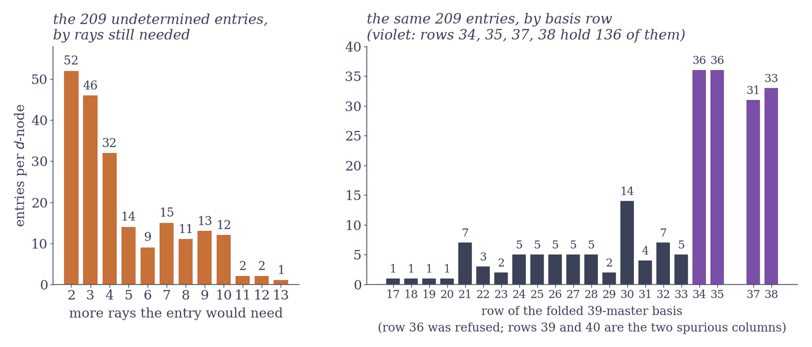
The 209 entries per $d$-node the first, 24-ray design left undetermined were a finding about the ray design, not a residue: the design counted the ray degree and not the pure factor, so each family needed 2 to 13 more rays, most of them (136, the violet bars) in rows 34, 35, 37 and 38. The widened 37-ray fit placed its 13 further rays by these degrees and determined all 209. Chart drawn for this page from the 24-ray fit of record; the counts are identical at the two $d$-nodes.
Downloads: lbl3x-expression.md · lbl3x-evaluate.py (--sector63-map checks, in exact rational arithmetic at the seven off-curve points, the two relations that carry the family's 41-master basis onto the 39-master one, from the reduction outputs shipped beside the script) · MANIFEST.sha256 (every file of the bundle with its checksum) · K3 seed constants · lower-block kernel · lower-block boundary · for --k3-words: K3 word list · $x_{17}$ constant record · for --theorem-check: kernel entry map · kernel denominators · kernel manifest, plus the witness files listed in the appendix. The evaluator reads every file from its own directory and the witness from lbl3x-kernel-witness/ beside it. lbl3x-k3letters-census.py reproduces the graded census of the K3 letters (179 leaves at order 3; a planted letter is refused, a duplicate absorbed) from the seven record objects it reads, pinned by sha under vendor_row21_k3letters/. Off the curve: row21_offcurve/ (the front end row21-offcurve-evaluate.py with the vendored chain legs, the 26 reductions gzipped — the seven of record and the 19 fresh regenerations, 75 MB of the folder's 281 MB — and the objects of record for rows 17–38; the default run reproduces the record's own rows-0–16 point in about half a minute and --leg chain the seven-point program in about seven minutes; --top prints the rows 17–38 figures of the 24-ray fit of record from the shipped objects (the 37-ray widening is not yet in the bundle) in about two seconds, --leg predict-top a withheld ray's prediction in about ten seconds, --leg residual-top --point all the residual tally over all 26 points in about twenty minutes, and --leg march-top one item of the march in about five minutes; --mutate-top is the planted control).
---
The ten-line parent (LBL3Q)
The family's open frontier is the diagram everything above descends from: the all-trivalent QED graph whose pinch the crossed box is — the ten-propagator non-planar fermion octagon with two crossed photon chords. It has not been computed; the crossed box above is its sector 938. Its top-sector geometry is established all the same: the maximal cut of the ten-line top sector is a non-isotrivial genus-one curve (thirty maximal-cut masters, $j(s,t)$ non-constant) — an elliptic curve intrinsic to the topology, where the elliptic curves of the sunrise and kite dressings and their QED parents above are all inherited from the self-energy sub-loop. We are not aware of a previously reported intrinsic curve in one-particle-irreducible light-by-light scattering. This is proven structure with no closure claimed; the earlier classification of the whole massive three-loop $\gamma\gamma\to\gamma\gamma$ hierarchy as genus-zero polylogarithmic is withdrawn, and LBL3Q is the natural next target.
Everything on this page was validated against independent evaluations at points never used in the construction, to at least 33 digits.
Tools
| Tool | Role |
|---|---|
| Kira + FireFly | integration-by-parts reduction, master bases, and differential equations for every member |
| AMFlow | the independent verification oracles, and boundary data |
| Eichler | the Γ₁(6) modular layer of the sunrise dressing |
| GeoTriage | per-sector geometry classification — the stratification that chose each route |
| Nestor | assembly of the dispersive one-folds with analytic threshold subtraction (Nestor's dispersion module) |
| Wayfinder | series transport of the differential equations (the spectral densities and the crossed box) |
| Numkin | exact reconstruction of the missing crossed-box connection entries |
| Lockpick | the lattice search certifying that no constant basis reaches the crossed-box finite piece |
| PSLQ | identification of boundary constants, and the decisive negatives |
Appendix: the kernel function-form refutation (LBL3X)
The sections above evaluate integrals; this one proves a negative and supplies the proof. The two are deliberately kept apart: the crossed-box evaluator above reads none of the data below, and nothing below is needed to reproduce the results above.
Theorem (no finite-depth function form in the raw frame). In the raw frame of the 41-master basis, the kernel system of the crossed box is not finite-depth: the strongly-connected condensation of its $\varepsilon^0$-graded support is a directed acyclic graph of depth four whose top component is a twenty-four-row block irreducibly coupled at $\varepsilon^0$. Evaluating the raw-frame system therefore requires the fundamental matrix of that block's $23\times23$ $\varepsilon^0$ core, and the system terminates as a finite Chen iterated integral only after an $\varepsilon$-factorised rotation of the block; the raw-frame form is a coupled Volterra system, not a finite-depth iterated integral. The separate negative for the top-sector master — no generalised-polylogarithm closed form for $m_{18}^{(0)}$ — stands independently of this theorem. The closed forms live in the connection that generates them: the $41\times41$ pair $(A^s,A^t)$ of exact bivariate rational functions of $(s,t)$. Its entries are the differential equation, not solutions of one — the pair is the definition of the object, and the witness below carries it exactly.
The certificate. The proof is data plus a checker. The statement is the paragraph above. The witness is the exact connection at one declared node of the reconstruction, byte-pinned (about 12.5 MB) — that one node carries the full exact $(s,t)$ content the theorem needs; the rest of the reconstruction scaffolding stays in the project archive. The checker is the evaluator's --theorem-check mode, which verifies the witness files byte-for-byte on load, confirms the coupling structure, evaluates any connection entry, and refuses loudly — naming the file and its pin — if the witness is absent or altered, rather than degrading to a partial answer. Of the 2,045 nonzero entries of the pair, 1,989 are exact rational functions (46 of them entered the exact bank on 7 September 2026, when 71 of the 97 two-prime columns were closed exactly by Chinese remaindering over five to nine primes and checked against both reconstruction primes' residues at every node), 16 are certified only as residues modulo the two reconstruction primes, and 40 remain unclosed — the checker names those rather than interpolating past them, and their only cure is denser reconstruction data. One structural fact must be stated: the raw $(A^s,A^t)$ pair is not a flat two-dimensional connection away from the transport curves (a frame defect of the raw source pair); the frame-clean object is the combination $V=A^s-(t^2/s^2)\,A^t$ along the foliation $1/s+1/t=\mathrm{const}$, and that is what every validated consumer of the connection uses. The reconstruction was cross-checked several independent ways with zero mismatches, including a full independent symbolic rerun; the crossing symmetry $s\leftrightarrow t$ is exact: the $41\times41$ crossing matrix $C(s,t,d)$ satisfies $C(s,t,d)\,C(t,s,d)=I$ identically in $\mathbb{Q}(s,t,d)$, the $39\times39$ matrix obtained by folding the two spurious sector-63 masters onto the thirty-nine by their reductions satisfies the same identity, and a crossing check of 40,854 exact comparisons on data kept out of the reconstruction returned zero mismatches, the involution holding at 10,086 of 10,086.
The obstruction, characterized. The residue eigenvalues of the full connection at $s=0$ are the roots of an irreducible cubic over $\mathbb{Q}$ (characteristic polynomial $11\lambda^3-175\lambda^2-326\lambda+760$), so the system is not $\varepsilon$-factorisable to dlog form. After an exact $\varepsilon$-rational rotation to the intrinsic banana frame, the K3 block's letter ring is six pulled-back $\Gamma_1(6)$ letters with no Eichler quadratures surviving in the block; the final assembled form of $m_{18}$ is not claimed.
Downloads: lbl3x-evaluate.py --theorem-check · witness slice_n1_exact.pkl.gz (12 MB) · slice_n1_fits.pkl.gz · manifest (byte-pinned) · kernel entry map
References
| Massless 3-loop γγ→γγ | P. Bargiela, A. Chakraborty, G. Gambuti, M. A. Ozcelik | arXiv:2603.22423 |
| Massive 2-loop γγ→γγ | Ajjath A H, E. Chaubey, H.-S. Shao | arXiv:2312.16966, JHEP 03 (2024) 121 |
| ATLAS observation | ATLAS collaboration | arXiv:1702.01625, Nat. Phys. 13 (2017) 852 |
| Sunrise on Γ₁(6) | L. Adams, S. Weinzierl | arXiv:1704.08895 |
| 3-loop massive γγ→γγ masters | This work | new |