Neutral biodiversity (ecology)
The content on this page was written by AI under human supervision.
On an island in the Panama Canal, every tree in fifty hectares of tropical forest has been counted eight times since 1982. The two papers summarized here use those counts to put neutral theory, in which species differ only by luck, to an exact test. They then build the smallest model that can predict which species will gain trees and which will lose them.
A forest observed, a forest deciphered — the story of this page told in seven minutes: thirty years of tree censuses on Barro Colorado Island, Panama, built by Smithsonian field crews and made public, test neutral theory exactly and show that measured life histories, seed arrival from the surrounding forest and shared good and bad years predict which species gain and lose trees, which are common, and how much the whole forest fluctuates. (Download the video, 14 MB.)
The island and the census
A fifty-hectare plot of forest on Barro Colorado Island was censused in 1982, again in 1985, and every five years from then through 2015: eight complete censuses over 33 years. In each one, field crews tag, identify and measure every free-standing woody stem at least one centimeter thick, and record which stems have died, grown or newly appeared since the census before. The first census found 235,360 living stems of 320 species. The first paper here uses only trees with trunks at least ten centimeters across: about 21,000 in each census, of 230-odd species (255 over all eight censuses).
Most species in the plot are rare: the commonest has about two thousand trees, but in the 2005 census 167 of the 230 species had 63 or fewer, and 22 had a single tree. The censuses also show each species gaining or losing trees from one census to the next. Part of that change is chance, which trees happen to die and which leave offspring; ecologists call that part driftchange in a forest’s mix of species produced by chance deaths and births alone, with no species favored. The rest reflects real differences among the species. Telling the two apart requires knowing exactly what chance alone would do.
Neutral theory
The lopsided pattern of a few common species and many rare ones had a statistical description long before it had an explanation. In 1943 the statistician R. A. Fisher and two colleagues proposed that, in a large sample, the number of species represented by exactly $n$ individuals is
$$S(n) \;=\; \alpha\,\frac{x^{n}}{n},$$
where $x$ is a number a little below one, set by the size of the sample, and $\alpha$, now called Fisher’s alpha, measures diversity. Species seen once outnumber those seen twice, and so on down a long tail.
Stephen Hubbell, an ecologist who developed his ideas largely on the Barro Colorado data, proposed a mechanism in 1997 and set it out fully in a 2001 book, The Unified Neutral Theory of Biodiversity and Biogeography. It is neutral in the sense that species do not matter: every tree, whatever its species, has the same chances of dying, of leaving offspring and of having arrived as a seed from outside. The plot holds a fixed number of trees, $J$. When one dies, its place goes with probability $m$ to a seed from the surrounding region, drawn in proportion to how common each species is out there. Otherwise it goes to the offspring of a tree already in the plot, picked at random. In the region, new species arise rarely and steadily, and regional abundances then follow Fisher’s log-series exactly, with Hubbell’s “fundamental biodiversity number” $\theta$ in the role of $\alpha$. Two numbers, $\theta$ and $m$, govern everything.
Hubbell wrote in the book itself that “the assumption of complete neutrality is patently false.” Ecologists adopted the theory anyway, for two reasons. It fits the abundance curves of many kinds of community with two or three numbers, whereas richer models fit no better and, when they miss, one cannot tell which ingredient is to blame. And it can be solved. The same mathematics had been worked out in population genetics, where Warren Ewens’s formula of 1972 gives the exact odds of any sample of gene variants drifting without natural selection. By 2005 Rampal Etienne had extended it to the probability of an entire census of Hubbell’s plot, and, as earlier fits had shown, the theory matches a single Barro Colorado census well. Neutral theory thus became community ecology’s working null modela deliberately simple theory used as a baseline: where real data depart from it, something the theory leaves out is at work: the prediction of chance alone, kept because its failures point to real biology.
Solving neutral theory exactly
Neutral theory comes in two forms. In the spatially implicit form just described, the plot is a well-mixed collection of $J$ trees taking in seeds from a large, featureless region. In the spatially explicit form every tree stands somewhere on a landscape and drops its seeds within a few tens of meters. How many seeds cross the plot’s edge then follows from the rules, with no immigration number left to adjust. The first paper solves both. For the implicit form it derives exact formulas for what repeated censuses measure, above all how much each species’ count should change between censuses by drift alone. For the explicit form, whose predictions for a plot’s species counts had come only from simulation or a 2018 approximation, it reduces the theory to one equation.
The reduction to one equation works because species in the explicit form never interact, so each species is a family tree descended from one founder. Let $\phi(x,s)$ be the probability that a tree standing at position $x$ a time $s$ ago has at least one living descendant inside the plot today. The expected number of species in a plot of area $A$ is then
$$S(A) \;=\; \nu\rho\int_0^{\infty}\! ds\!\int\! d^{2}x\;\phi(x,s), \qquad\qquad \frac{\partial\phi}{\partial s} \;=\; D\,\nabla^{2}\phi \;-\; \nu\,\phi \;-\; b\,\phi^{2}.$$
Here $\rho$ is the density of trees and $b$ a tree’s birth rate. New species arise at the small rate $\nu$, matched by a slight excess of deaths over births, and $D = b\sigma^2$ sets how fast a line of descent wanders when seeds land a typical distance $\sigma$ from their parent. The first relation adds up, over every place and past moment at which a founder could have appeared, the chance that its line survives into the plot now. The second says how that chance changes as one looks further back: its three terms spread the lineage by seed dispersal, thin it by the excess deaths, and account for the branching of the family tree. A variant of the equation gives the expected number of species at each abundance, which the authors solve numerically to a stated accuracy.
The tree density comes from the census; the explicit form’s two remaining inputs, the seed distance $\sigma$ and the speciation rate $\nu$, had been fitted earlier, in 2002 and 2018, to a different kind of data: how quickly the species makeup of Panama’s forests changes with the distance between plots. The fitted seed spread is about 40 meters along each axis ($\sigma \approx 28$ m in the equation above). With those values, the 2005 tree count, and nothing adjusted to this plot, the full solution expects 82 species among trees at least ten centimeters thick, give or take 9, and 1.4 species present as a single tree. The census found 230 and 22. At the same inputs the 2018 approximation gives 47 and 0.7, so the exact answer roughly doubles the expected counts without coming near the census, and no inputs consistent with the Panama data do much better. The shortage of rare species is a property of the theory itself: a neutral forest whose seeds fall near their parents cannot hold nearly as many rare species as this one.
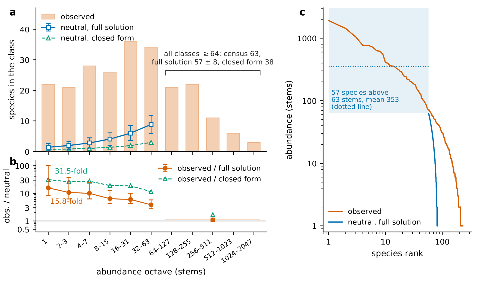
The 2005 census against neutral theory solved in full. (a) Bars: species in each abundance class among trees at least ten centimeters thick (230 species, 20,850 trees), the classes doubling in width from single-tree species at the left. Blue squares: what the spatially explicit theory expects, class by class, from the full solution of its one equation, with dispersal and speciation set by earlier fits across Panama and nothing adjusted to this plot; error bars are the theory’s own chance spread. Green triangles: the 2018 approximation. Above 63 trees the solution gives only a total (bracket). (b) Observed divided by expected, on a logarithmic axis where 1 means agreement. (c) The census (orange) and the solution (blue) as rank–abundance curves: trees per species, from the commonest species to the rarest. Solved exactly, neutral theory gives this plot far too few rare species, 82 species where 230 were counted and 1.4 single-tree species where 22 were; only the pooled count of common species comes close (63 counted, $57 \pm 8$ expected). (Figure from the first paper.)
The second comparison with the censuses uses change over time. Under drift a species’ count takes a random walk, one tree at a time, and the solved theory says how far it should wander. A species with $n_t$ trees at one census should show by the next a squared change that averages about
$$\mathbb{E}\big[(n_{t+1}-n_t)^{2}\big] \;\simeq\; \frac{2K\,n_t}{J}\Big(1-\frac{n_t}{J}\Big),$$
where $K$ is the number of trees that died and were replaced between the two censuses. The expected change grows in proportion to abundance because drift acts on one tree at a time; a cause acting on a whole species at once, a run of dry years, say, would give the square of abundance instead. Across the eight censuses the observed changes exceed the neutral expectation at every abundance, by two to six times for most species. The commonest may overshoot the most, though that hint rests largely on two species with long steady trends. Overall, the mix of species changes about as fast as drift would change it if trees were replaced four times as often as they are. It was already known that abundances at Barro Colorado change faster than drift allows; the exact solution gives the excess a definite size at every abundance. The authors assign no cause in the first paper and search for one in the second.
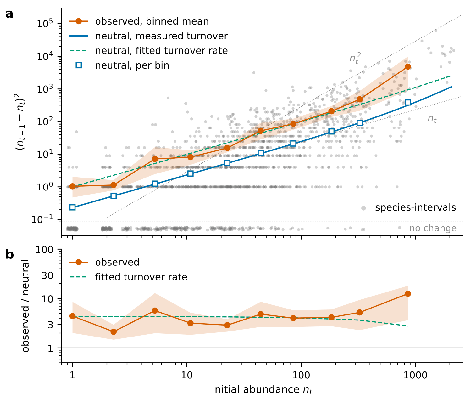
How much species’ tree counts change from one census to the next, against how many trees they started with (eight censuses, 1982–2015, trees at least ten centimeters thick). (a) Mean squared change per census interval in doubling bins of starting abundance $n_t$. Orange circles and band: observed, with a 95% range. Gray dots: single species over single census intervals; those whose count did not change are gathered in the row along the bottom. Blue line and squares: the exact neutral expectation at the deaths and replacements actually recorded. Green dashes: neutral drift speeded up to the replacement rate that best fits the observed changes (see text). Dotted guides: growth in proportion to $n_t$ (drift) and to $n_t^2$ (a cause acting on a whole species at once). (b) Observed divided by neutral. Abundances change several times more than drift allows at every abundance, among rare species and common ones alike. (Figure from the first paper.)
After neutral theory
A theory that treats species alike can never predict which species will gain trees and which will lose them. The second paper asks how little must be added to the neutral lottery before a model can. The authors’ answer is to let species differ in the one way the censuses measure directly: their life histories, meaning how fast their trees grow, how long they survive and how many young they leave. Kenneth Jops, James Dalling and James O’Dwyer tabulated those rates from these censuses in 2025, for each species in eight size classes, inferring seed output from the size at which a species first reproduces. The model follows 84 species, each climbing its own ladder of sizes at its own rates. The censused stems of those species are capped, all together, at their average count, about 200,000; when one dies, a waiting seedling of any species, drawn by lot, takes its place. Seeds also arrive from outside in proportion to each species’ share of plots elsewhere in Panama. Finally, measured sapling growth ran fast for nearly every species at once in the 1980s, slow in the 1990s and near average since. So each census interval gets one random factor, shared by every species, that speeds or slows the growth of small trees; its strength is measured from the sapling records, not tuned to any abundance.
The model’s first test is the forecast one could have made in 1995. Rates re-measured from the first four censuses alone are applied to each species’ standing mix of small and large stems in 1995, 2000 and 2005. They predict its change in large trees (trunks about eight centimeters and up) five and ten years on. Predicted and observed changes have a rank correlationa correlation computed on the ordering of species rather than on their values, asking only whether two quantities rank the species the same way; 1 is a perfect match, 0 none of 0.71 one census ahead and 0.68 two censuses ahead, well above simply extending each species’ past trend (0.54). The forecast works because a species with many saplings just below large-tree size is about to gain large trees, whatever it did before. Under neutral theory nothing measured early could rank the later changes, yet the 1980s size structures rank the species’ changes from 1990 to 2015 with a correlation that none of 600,000 simulated neutral forests and reshufflings reaches.
The model’s second test is the long run. Run for thousands of model years, the model settles into a steady mix of species. In that mix each species’ number of large trees is its seed arrivals times its local gain, the large trees its life history yields per arriving seed. With seeds arriving by regional abundance alone, the species come out in roughly the right order (rank correlation 0.67): the locally common species are the regionally common ones. The amounts are wrong, though, with far too many trees for species whose seedlings most often reach large size. The alternative weights each species’ arrivals down by its local gain, so that strong competitors are weak colonizers, an old idea in ecology called the competition–colonization trade-off. That brings the amounts close as well, and the abundance curve nearer the census than a fitted neutral curve. The authors call this a phenomenological repair, since nobody has yet measured which seeds actually arrive.
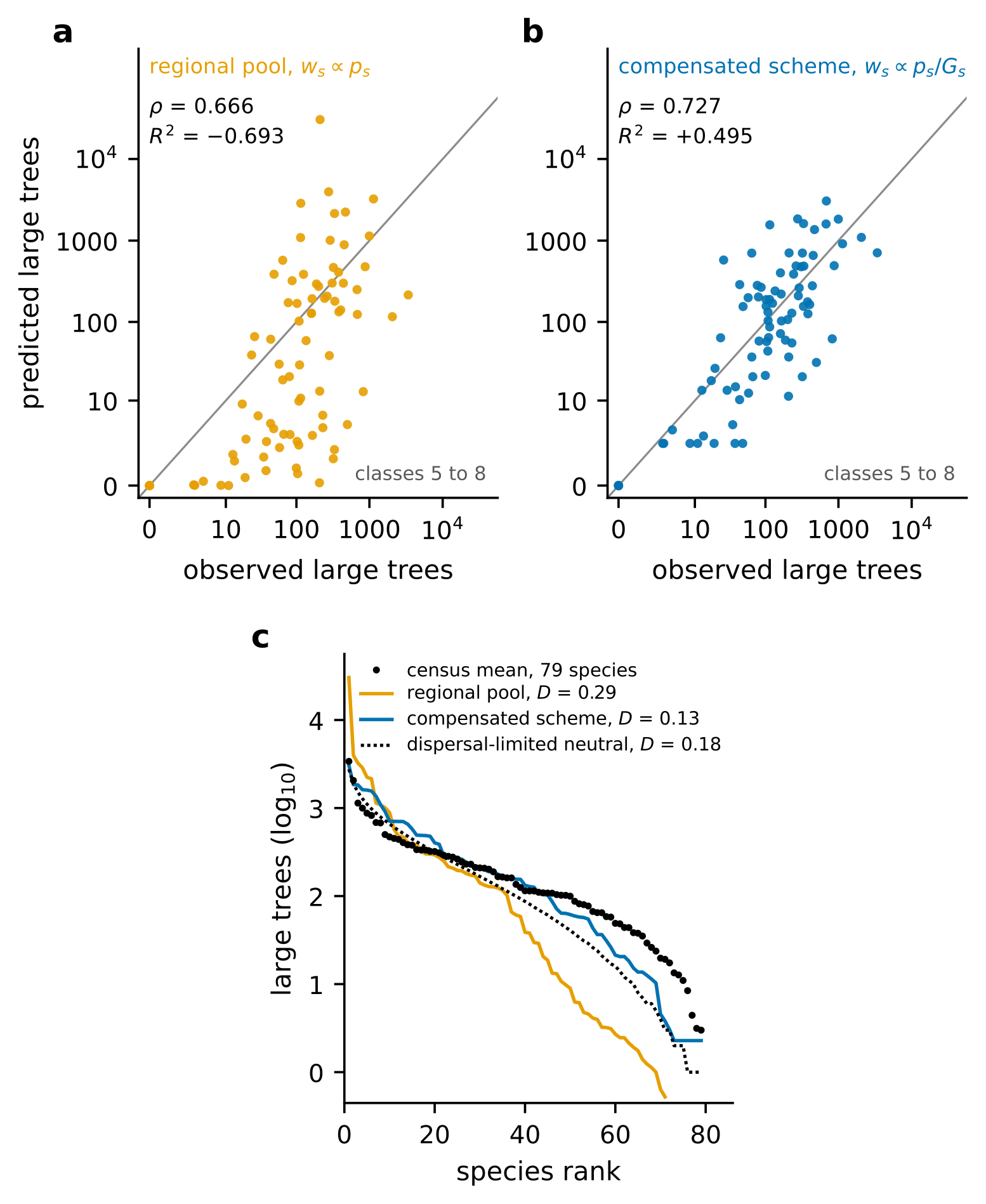
The minimal model’s long-run number of large trees for each species against the 1982–2015 census means, one point per species on logarithmic axes, the gray line marking perfect agreement. (a) Seeds arriving in proportion to regional abundance alone: roughly the right order, badly scattered amounts (rank correlation 0.67, $R^2 = -0.69$ against the line). (b) Arrivals also weighted against each species’ local gain, the competition–colonization trade-off: rank correlation 0.73, $R^2 = +0.50$. (c) The same predictions as ranked abundance curves, census in black, with a neutral curve fitted to the same species dotted (the 79 that reach large-tree size); $D$ measures how far each curve’s distribution of abundances lies from the census’s, zero meaning identical. Regional commonness sets which species are common, and the trade-off brings the amounts close, closer than a fitted neutral curve. (Figure from the second paper.)
The shared good and bad years matter most for the forest as a whole. Without them the model forest is twelve times too steady from census to census; with them the flow of trees into the large size classes varies about as much as it really does. One number per interval produces different swings in different species because each has a different share of its stems at sapling size at the time. Species of middling abundance still change two to three times too little in the model, which also ranks the species poorly among seedlings and small saplings.
What is settled and what is open
Both departures from neutral theory at Barro Colorado, too few rare species and abundances that change faster than drift allows, were reported before; the first paper pins down their size, which any richer model of this forest must now reproduce. Everything here concerns one well-studied forest, and the first paper one size class of trees. In the second paper the authors do not identify what drives the shared swings in sapling growth, since no climate record they examined tracks them beyond chance (though seven intervals cannot rule one out), and they had to assume how long the swings persist. The model’s forecasts run high in absolute numbers, and its long-run amounts hold only if every species exactly replaces itself over time. Whether a model this simple describes other forests has not been tried.
The papers
- Neutral biodiversity theory solved and tested against three decades of Barro Colorado censuses — Matthew D. Schwartz (Harvard) and James P. O’Dwyer (Illinois); in preparation, not yet posted. Solves neutral theory in its spatially implicit and spatially explicit forms and tests both against the Barro Colorado censuses.
- A minimal model of a forest after neutral theory (PDF) — Matthew D. Schwartz (Harvard) and James P. O’Dwyer (Illinois); the version hosted here is marked preliminary. Builds the minimal life-history model and tests its forecasts, its long-run abundances and its census-to-census fluctuations against the same censuses.
- Predicting the life history of forests — a third paper, in preparation.
Supplementary material
Every dataset the papers analyze is public. The tree censuses both papers rest on are listed below; each paper’s data statement lists the other datasets it uses and states the authors’ plans to archive their code.
- Supplementary material (PDF) — the second paper’s supporting information, in ten sections: the species and data; the stationary state and the simulations; the shared year effect estimated from the recorded stem transitions; alternatives set aside; the decadal forecast test in detail; a test of neutral drift at Barro Colorado; the long-run composition in detail; the fluctuation predictions; the seedling pool by species; and the data sources and code archive.
- doi:10.15146/5xcp-0d46 — the complete 1982–2015 censuses of the Barro Colorado 50-hectare plot (R. Condit, R. Pérez, S. Aguilar, S. Lao, R. Foster and S. Hubbell, 2019), archived on Dryad; the tree counts both papers analyze.
References
| R. A. Fisher, A. S. Corbet and C. B. Williams, The relation between the number of species and the number of individuals in a random sample of an animal population, J. Anim. Ecol. 12 (1943) 42 | the log-series law of species abundance and Fisher’s alpha |
| W. J. Ewens, The sampling theory of selectively neutral alleles, Theor. Popul. Biol. 3 (1972) 87 | the exact odds of a sample of gene variants drifting without selection |
| D. Tilman, Competition and biodiversity in spatially structured habitats, Ecology 75 (1994) 2 | a spatial model of the competition–colonization trade-off |
| S. P. Hubbell, A unified theory of biogeography and relative species abundance and its application to tropical rain forests and coral reefs, Coral Reefs 16 Suppl. (1997) S9 | Hubbell’s unified neutral theory proposed |
| S. P. Hubbell, The Unified Neutral Theory of Biodiversity and Biogeography, Monographs in Population Biology 32, Princeton University Press (2001) | the theory set out in full, with its two numbers $\theta$ and $m$ |
| J. Chave and E. G. Leigh, Jr., A spatially explicit neutral model of β-diversity in tropical forests, Theor. Popul. Biol. 62 (2002) 153 | the spatially explicit form, with seeds falling near their parents |
| R. Condit et al., Beta-diversity in tropical forest trees, Science 295 (2002) 666 | species similarity against distance across Panama; source of the fitted seed distance and speciation rate |
| I. Volkov, J. R. Banavar, S. P. Hubbell and A. Maritan, Neutral theory and relative species abundance in ecology, Nature 424 (2003) 1035 | an early fit showing that the theory matches a single Barro Colorado census |
| R. S. Etienne, A new sampling formula for neutral biodiversity, Ecol. Lett. 8 (2005) 253 | the exact probability of an entire census of Hubbell’s plot |
| R. A. Chisholm et al., Temporal variability of forest communities: empirical estimates of population change in 4000 tree species, Ecol. Lett. 17 (2014) 855 | showed that abundances at Barro Colorado and elsewhere change faster than drift allows |
| J. P. O’Dwyer and S. J. Cornell, Cross-scale neutral ecology and the maintenance of biodiversity, Sci. Rep. 8 (2018) 10200 | the 2018 approximation to a plot’s species counts in the spatially explicit form |
| K. Jops, J. W. Dalling and J. P. O’Dwyer, Life history is a key driver of temporal fluctuations in tropical tree abundances, Proc. Natl. Acad. Sci. USA 122 (2025) e2422348122 | the life-history rates by size class that the second paper’s model uses |