Phylogenetics (evolutionary biology)
The content on this page was written by AI under human supervision.
For a handful of species, Bayesian phylogenetics can score each candidate family tree by one number, the marginal likelihood: the probability of the observed DNA under that tree, averaged over a prior distribution on the unknown branch lengths. The same number is also used to compare models of DNA change. Since the 1990s it has been estimated by Monte Carlo simulation. Two papers by Matthew D. Schwartz, Scott V. Edwards and Paul O. Lewis show that for four or five species, under the simplest models of DNA change, it is an exact fraction, computable with techniques developed for Feynman integrals in particle physics. The first paper establishes the method; the second describes software that performs the computation and labels every value it returns with the kind of number it is.
Trees and the marginal likelihood
A phylogenetic tree records which species descend from which common ancestors, and today it is inferred largely from molecular data: DNA accumulates substitutions over time, so species whose sequences differ little parted recently. Line up the same gene from several species, one row per species and one column per position. A column in which human and chimpanzee share one letter while gorilla and orangutan share another supports grouping human with chimpanzee.
Four species can be joined into an unrooted tree (one that records the branching but not where the deepest ancestor sits) in exactly three ways, and five species in fifteen. At these sizes every candidate can be written down and scored. Bayesian phylogenetics, introduced in the late 1990s and now standard, scores a tree topology $T$ by its posterior probability, which for equally weighted trees is proportional to the marginal likelihood, or evidence:
$$ Z(T\mid u) \;=\; \int p(u\mid T,t)\,\pi(t\mid T)\,\mathrm{d}t . $$Here $u$ is the alignment, summarized by how many columns show each pattern of agreement; $t$ is the list of branch lengths, in expected substitutions per site; $p(u\mid T,t)$ is the probability of the data given the tree and its branch lengths, computed by Felsenstein’s pruning algorithm of 1981; and $\pi(t\mid T)$ is a prior on the branch lengths. The ratio of two trees’ marginal likelihoods is a Bayes factorThe ratio of the marginal likelihoods of two hypotheses; here, of two trees or two substitution models. Both papers report its natural logarithm, in “log units” (nats). A log Bayes factor of 3 is the conventional threshold for strong evidence., and its natural logarithm gives the “log units” in which both papers report every comparison.
Why the integral has always been estimated
The integral has one dimension per branch, five for a four-species tree, or quartet, and has been regarded as analytically intractable for all but trivial cases. In 1996 Rannala and Yang obtained posterior probabilities for four hominoid species by direct numerical integration, an approach limited to about five taxa, as the tips of a tree are called. For larger trees the integral is estimated from the output of a Markov chain Monte Carlo sampler that wanders through branch-length space. Thermodynamic integration (brought to phylogenetics in 2006) and stepping-stone samplingAn estimator (Xie and colleagues, 2011) that climbs from the prior to the posterior through a ladder of intermediate distributions, each proportional to the prior times the likelihood raised to a power β between 0 and 1, and multiplies together the estimated ratios between neighboring rungs (“stones”). Thermodynamic integration instead integrates the average log-likelihood along the same ladder by a quadrature rule. (2011) are the estimators now in standard use, the latter built into MrBayes, RevBayes and BEAST; LoRaD (2023) is a recent addition. In 2020 Fourment and colleagues compared nineteen such methods, under the title “19 dubious ways to compute the marginal likelihood of a phylogenetic tree topology.”
Earlier comparisons of marginal-likelihood estimators shared one limitation: the reference value was the analytic answer of a textbook model that is not a tree, or another estimator, or a very long run of the same sampler. In none of them was it an exactly known marginal likelihood of a tree on real sequence data, so each program’s run-to-run scatter was known but its distance from the true value was not.
The integral is a fraction
The simplest model of DNA change is the Jukes–Cantor model of 1969: every letter mutates to each of the other three at the same rate. Along a branch of length $t$, the probabilities that a site keeps its letter, or ends with one particular different letter, are
$$ P_{\text{same}}(x) \;=\; \tfrac14 + \tfrac34\,x, \qquad P_{\text{different}}(x) \;=\; \tfrac14 - \tfrac14\,x, \qquad x \;=\; e^{-4t/3}. $$The variable $x$ runs from 1 for a branch of zero length to 0 for an infinitely long one, and both probabilities are linear in it. Pruning multiplies one such factor per branch and sums over the unknown letters at the two internal nodes. The probability of any column is therefore a polynomial in the five branch variables $x_1,\dots,x_5$, of degree at most one in each, with integer coefficients divided by 256. Because the model treats the four letters alike, the 256 possible columns collapse into fifteen pattern classesThe set partitions of four species by shared letter: xxxx (all agree), xxyy (species 1 and 2 agree against 3 and 4), xxxy (only species 4 differs), and so on down to xyzw (all four differ). An alignment enters the computation only through the fifteen counts of columns in each class.. MrBayes and RevBayes offer an independent exponential prior on each branch length; at rate $4/3$ (mean 0.75 substitutions per site) the change of variables makes it uniform in $x$. The evidence becomes the integral of a polynomial over the unit cube, taken one term at a time:
$$ Z(T\mid u) \;=\; \int_{[0,1]^5} \prod_{k=1}^{15} p_k(x)^{u_k}\,\mathrm{d}x_1\cdots\mathrm{d}x_5 \;=\; \frac{1}{256^{N}} \sum_{a} c_a \prod_{e=1}^{5} \frac{1}{a_e+1} . $$On the left, $p_k$ are the fifteen class polynomials and $u_k$ the observed counts for an alignment of $N$ columns. On the right, the product has been expanded into monomials $x_1^{a_1}\cdots x_5^{a_5}$ with integer coefficients $c_a$, and each power $x^{a}$ replaced by its integral over the unit interval, $1/(a+1)$. A finite sum of fractions is a fraction. That is Lemma 1 of the first paper, and its proof is the algorithm, traced in the figure below. The same argument covers any exponential prior of rational rate, Kimura’s 1980 two-parameter model and, by a different route, any time-reversible model, once the extra rate parameters and base frequencies are fixed at rational values.
![Four-panel vertical schematic. (a) A twenty-column alignment of four rows labeled taxon 1 to taxon 4, letters A C G T, with columns tinted by pattern class: gray for all-agree, blue for 12 versus 34, orange for 13 versus 24, green for 14 versus 23, pink for one-differs, yellow for all-differ. An arrow labeled count the site patterns leads to (b): an unrooted four-leaf tree with leaves 1, 2, 3, 4, pendant edges x1 to x4 and internal edge x5, the formula x_e equals e to the minus mu t_e in [0,1], and a table of pattern counts xxxx 10, xxyy 4, xyxy 2, xyyx 2, xxxy 1, xyzw 1, N equals 20, nine other classes 0. An arrow labeled one polynomial per pattern, by pruning leads to (c): the polynomial 256 p_xxyy(x) equals 1 plus 3 x1 x2 plus 3 x3 x4 plus 9 x1 x2 x3 x4 minus four cubic terms minus twice four quartic terms minus 4 x1 x2 x3 x4 x5, and the integral Z(12|34) over the unit five-cube of p_xxxx to the 10, p_xxyy to the 4, p_xyxy squared, p_xyyx squared, p_xxxy, p_xyzw. An arrow labeled expand; each monomial gives integral of x to the a equals 1 over (a plus 1) leads to (d): Z(12|34) equals n over d exactly, with n a 49-digit integer beginning 8390002712 and d an 87-digit integer beginning 9757640891, and log Z(12|34) equals minus 87.649243349.](/img/phylo-schematic.png?v=b3e6e7c477)
From alignment to fraction, on the first paper’s twenty-column worked example. The columns of a four-species alignment (a) are sorted into pattern classes and counted (b). Pruning turns each class into a polynomial that is linear in each of the five branch variables $x_e$ (c, shown for the class in which species 1 and 2 agree against 3 and 4). The likelihood is the product of these polynomials raised to their counts; under the uniform prior on each $x_e$ every monomial integrates to a product of reciprocals of whole numbers, so the evidence is one explicit integer over another (d). No step involves a random number or a rounding. (Figure 1 of the first paper.)
Expanding the product of class polynomials is expensive, however: up to $(N+1)^5$ monomials, with coefficients hundreds of digits long. Most columns in a real alignment are constant or support the tree being scored, and those factor out cheaply; only the $m$ mixedA column is mixed, for the tree being scored, if it is neither constant nor of the one class that supports that tree (species 1 and 2 sharing one letter and 3 and 4 another, for the tree pairing 1 with 2). Constant and supporting columns factor out of the computation cheaply; mixed columns do not. columns need the full expansion, so the cost scales as $N(m+1)^5$. Every step runs in modular arithmetic, a technique taken from the exact evaluation of Feynman integrals (von Manteuffel and Schabinger, 2015). The computation is repeated modulo several primes just below $2^{31}$, and the Chinese remainder theorem reassembles the exact integer with no floating-point operation anywhere. In the variables $x_e$ the evidence has the form of a Feynman integral in parametric representation, which algebraic statisticians call a GKZ hypergeometric integral.
The first paper’s reference alignment is the mitochondrial transfer-RNATransfer RNAs are short adapter molecules, roughly 70 to 90 nucleotides long (mitochondrial ones run shorter), that carry amino acids to the ribosome during protein synthesis. Their genes are among the shortest there are, short enough for the exact computation. gene tRNA-Gln in mouse, rat, chicken and the frog Xenopus: 68 columns, 25 of them mixed for the mouse–rat tree (32 and 33 for the other two trees). Each of its three evidences is a ratio of integers of roughly 190 and 300 digits, and the tree pairing mouse with rat wins by 14.54 and 15.56 log units, the accepted answer. On 72 cores, all three took about three times the elapsed time of a single-core MrBayes run (one to two hundred times its processor time, the higher figure counting a deliberate duplicate evaluation of every value on a second set of primes); two classic 900-column alignments, with hundreds of mixed columns, remain out of reach. Exactness also has limits; if columns are allowed to evolve at different rates (gamma-distributed rate variation across sites), three species and a single constant column at gamma shape 1 already give $(10-6G)/64$, with $G = 0.5963\ldots$ the Euler–Gompertz constant: computable to any precision, but presumably irrational.
An exact tie among the great apes
A second transfer-RNA gene, tRNA-Phe, in human, chimpanzee, gorilla and orangutan, gives the clearest example of a fact that no Monte Carlo estimate can establish. The alignment has 69 columns, 59 constant and 10 carrying a change private to one species, none grouping two apes against the other two. Computed separately, the evidences of the human–chimpanzee tree and of the chimpanzee–gorilla tree came out as the same 217-digit integer over the same 287-digit integer. The tie follows from a symmetry that played no part in the computation: swapping the labels “human” and “gorilla” leaves every pattern count unchanged and carries one tree into the other. The third tree, pairing human with gorilla, maps to itself under the swap and is tied to neither. It has the largest evidence of the three, by 0.0013 log units, although no column supports it; the authors interpret this small margin as the prior’s apparent preference for joining the two most similar sequences. Stepping-stone runs on this alignment scatter by 0.017 to 0.067 log units, and no finite sample can show a difference to be exactly zero.
Adding the gibbon gives fifteen trees, and the first paper computes all fifteen exactly. The swap still preserves the counts, so twelve trees fall into six exactly tied pairs. The top value, $\log Z = -189.6451$, is shared by the accepted hominoid tree, with human and chimpanzee paired and orangutan and gibbon paired, and its mirror with chimpanzee and gorilla paired. The human–gorilla resolution that nominally won at four species now ranks third, 0.5625 log units behind. The two columns where human and gorilla differ have become informative, and both count against joining them.
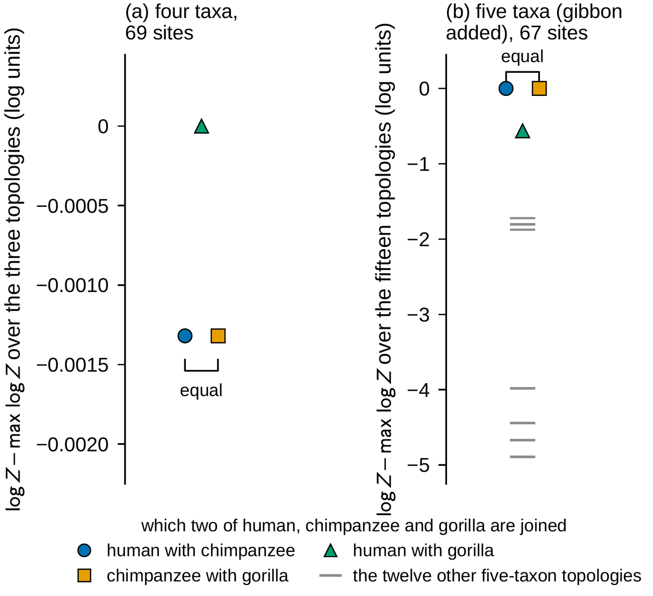
The three ways to resolve human, chimpanzee and gorilla, scored exactly without and with the gibbon. Each symbol is one tree’s exact log evidence relative to the best tree (Jukes–Cantor model, exponential branch-length priors of mean 0.75, equal prior weight on trees); “equal” joins values that are identical as ratios of integers, as the human–gorilla label swap requires. Left, the four-ape quartet: the human–gorilla tree leads by 0.0013 log units and the other two tie. Right, all fifteen five-ape trees on the same gene: the accepted tree and its mirror tie at the top and the human–gorilla tree falls 0.5625 log units behind. Note that the two vertical scales differ by more than a thousandfold. (Figure 5 of the first paper.)
Testing the estimators against the answer
Against the exact values, the first paper measures the estimators’ accuracy, with sampler settings fixed beforehand (figure below). On the tRNA-Gln quartet, MrBayes, RevBayes and LoRaD all come within a few hundredths of a log unit of the exact value. The MrBayes means, however, sit below the exact values on every tree. Longer chains and more stones remove part of the gap; a residual of −0.016 log units does not move and is common to the three trees. It disappears when one of MrBayes’s three default branch-length proposals, the node slider, is switched off: from version 3.2.4 onward that move’s proposal ratio contains one extra factor of the ratio of new to old tree length, so that, run without data, it samples trees 1.4 to 3 times longer than the prior mean. The offset cancels in these Bayes factors and is far below any threshold used to interpret one, but nothing MrBayes reports reveals it; a much longer MrBayes run, used as the reference, would make the other two programs look biased instead. RevBayes errs with both signs and converges toward zero as the budget grows; LoRaD agrees within its chain-to-chain spread.
A second test distinguishes two estimators that are fed the same samples. On a three-species, eight-column alignment the authors compute every ratio along a four-stone stepping-stone path without sampling. Stepping-stone sampling reproduces the exact $\log Z = -29.4932$ within Monte Carlo error at every budget. Thermodynamic integration over the same four intervals comes out low by 0.0095 log units, 39 standard errors at the largest budget: the trapezoidal rule misses the curvature between so few stones, and sampling longer at each stone does not help.
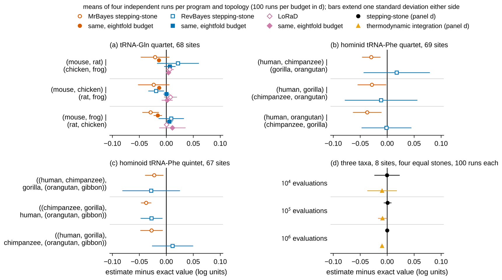
Estimators measured against exact values. Each symbol is the mean of independent runs minus the exact log evidence, with bars of one standard deviation; zero marks the exact value. Panels (a)–(c) are the tRNA-Gln quartet, the four-ape tRNA-Phe quartet and the three leading five-ape trees: MrBayes stepping-stone (orange) sits slightly low everywhere, while RevBayes (blue) and, in panel (a), LoRaD (pink) straddle zero. Panel (d) is the three-species, eight-column case on a four-stone path whose every ratio is known without sampling: stepping-stone (black) is unbiased within Monte Carlo error at each budget while thermodynamic integration (yellow) keeps a fixed shortfall as its scatter shrinks. Against an exact reference, a systematic offset can be told apart from Monte Carlo noise. (Figure 4 of the first paper.)
Beyond one gene: a tortoise and the malaria mosquitoes
The first paper ends with two applications. Jensen and colleagues (2022) placed the extinct San Cristóbal giant tortoise of the Galápagos, from one stretch of mitochondrial DNA (a locus) of about 700 nucleotides, as sister to two other Chelonoidis species with posterior probability 1.0. Under a design fixed in advance, the test statistic was the sum of twelve exact log Bayes factors for the published grouping, over two quartets and six segments of the locus. Confirmation required a sum of at least 3.0 with both quartet sums of the same sign. The observed sum is 0.90, and the two quartets disagree in sign, −3.61 and +4.51. Post-mortem DNA damage does not explain the shortfall: 150 replicates with such damage introduced all score below −43. The authors state that this does not show the published placement, which rests on a molecular-clock analysis of 93 distinct sequences, to be wrong; only that this locus, read this way, does not confirm it.
In the Anopheles gambiae complex of African malaria mosquitoes, Fontaine and colleagues (2015) found one species grouping differently on the autosomes (the non-sex chromosomes) and on the X chromosome. The first paper rebuilt their sliding-window scan in floating-point arithmetic, 81,113 windows on three quartets each, taking no position on gene flow, and recovered the reversal. It then computed exact values for the 5,375 window–quartet pairs within two size limits set in advance. Of these, 2,997 are exact ties, which floating point can break only by rounding error. Among the 2,378 with a unique exact winner, floating point picks the same tree in all but four, and those four are separated by at most 0.016 log units.
JaCK & Jill: the method as software
With the second paper the computation is released as a Python package, phyloexact version 0.2.3, named JaCK & Jill: JaCK for the exact Jukes–Cantor and Kimura computations, Jill for the interval and sampling routines. Given an alignment, a topology and a model, one call returns a marginal likelihood as one of four kinds of answer and reports which. An exact value is the fraction itself, under Jukes–Cantor for alignments about the length of a transfer RNA and under Kimura’s model for shorter ones. A proven interval brackets the value under the richer HKY85 and GTR+Γ models at fitted parameters, given enough computing time (a short run may prove only an upper bound). An estimate, by quasi-Monte Carlo importance sampling, works at any length; on small Jukes–Cantor quartets it comes with an error figure of 0.014 log units derived from deviations measured against exact values (an indicative accuracy, the paper says, not a bound). A proof of a tie is a permutation of the taxa that preserves the pattern counts and carries one topology into the other. Every answer comes with a machine-readable record that an independent routine rechecks against the alignment.
The exact values are then the reference for a benchmark on nine problems: the three trees each of the tRNA-Gln and four-ape tRNA-Phe quartets, and the three leading five-ape trees (figure below). At 2.5 million likelihood evaluations the phyloexact estimate misses by 0.0001 log units on average. On the three tRNA-Gln trees MrBayes stepping-stone sampling misses by about 0.024 and RevBayes by about 0.017, where phyloexact misses by 0.0003; LoRaD, run on the quartets, misses by about 0.005. Per single-thread run at that budget they take roughly 7 to 13 seconds against 31 for uncompiled phyloexact. The like-for-like comparisons favor phyloexact more strongly: at its default budget it runs in about four seconds per problem (about one second with the optional compiled kernel) with a mean error of 0.0006 log units. At equal run time, about 7 seconds, its error is 20 to 44 times below LoRaD’s and 67 to 213 times below the two stepping-stone programs’. To reach phyloexact’s default accuracy LoRaD would need about 500 seconds per run and RevBayes about 12,000, while MrBayes does not reach it at any budget because of the offset described above. The best of the nineteen methods from the 2020 comparison, all run in the program physher, reaches 0.0026 log units at twenty times the budget, 26 times the phyloexact error. For scale, against the conventional Bayes-factor threshold of 3 log units the stepping-stone and LoRaD errors are negligible, while thousandths of a log unit can matter where two values nearly tie and where one-signed errors accumulate over many loci.
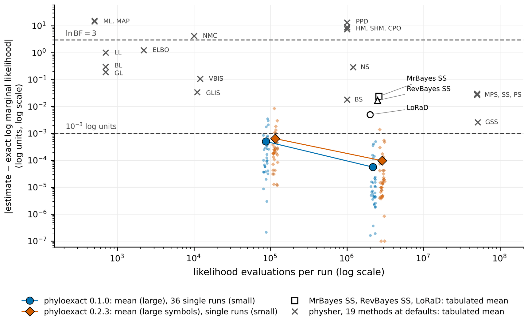
Error against the exact answer versus computing budget, on the nine transfer-RNA problems with exactly known marginal likelihoods. Crosses are the nineteen estimators of the 2020 comparison (program physher) at their default budgets; open symbols are MrBayes and RevBayes stepping-stone sampling and LoRaD; large filled symbols are the phyloexact estimate (orange diamonds, the released version 0.2.3; blue circles, an earlier release), with small points for single runs. The upper dashed line is the conventional strong-evidence threshold of 3 log units; the lower one marks a thousandth of a log unit. At a matched budget the package’s estimate sits one to two orders of magnitude below the programs in everyday use, and every point is a measured distance from the exact value rather than a self-reported spread. (Figure 3 of the JaCK & Jill paper.)
The package scores a given topology and does not search over trees. For five or more taxa it offers only the Jukes–Cantor estimate and tie proofs (for up to 32 taxa), and computes no exact five-taxon value. It runs 38 validation tests with one command and is free software under the MIT license.
What is settled and what is open
Two results are settled, both under the stated model and prior: for four and five species under Jukes–Cantor with independent exponential branch priors, the marginal likelihood is an exactly computable fraction, and the estimators in everyday use now have an absolute reference on real sequence data. The authors list what remains open: nearly every exact value on real data is a Jukes–Cantor value with at most 59 mixed columns; with rate variation across sites, which most published analyses include, the integral is no longer a finite sum of fractions; six species, with 105 trees, have not been attempted. For trees of realistic size Monte Carlo remains necessary, and the exact values serve as a check on it.
The papers
- Exact Bayesian evidence for phylogenetic trees (PDF) — Matthew D. Schwartz, Scott V. Edwards and Paul O. Lewis; currently marked preliminary. Establishes the method and works the examples above: the proof that the evidence of a four- or five-species tree under the Jukes–Cantor model is an exact fraction, the transfer-RNA quartets and the great-ape tie, the tests of the estimators against the exact values, and the tortoise and mosquito applications.
- JaCK & Jill: exact marginal likelihoods for small phylogenetic trees (PDF) — the same authors; currently marked preliminary. Describes the phyloexact package (version 0.2.3), its four kinds of answer, and the benchmark against MrBayes, RevBayes, LoRaD and the nineteen methods of the 2020 comparison.
Three application papers that earlier appeared on this site were withdrawn for revision in September 2026.
Supplementary material
Files hosted on this site. The two Python scripts recompute their values live rather than printing stored digits.
- Supplementary material (PDF) — the supplement to the first paper: rate variation across sites and the limits of exactness, recurrences in the pattern counts, the three evaluation programs with their measured cost and cross-checks, the deterministic stepping-stone path and the source of the MrBayes offset, the tortoise protocol and the mosquito window scan in full, and the exact values in machine-readable form.
- Supplementary material (PDF) — the phyloexact 0.2.3 manual: installation and a first session, every call with its options, returned objects and refusals, the models available for each kind of answer, the error statement of the estimate, cost planning, the full benchmark tables, and the format of the machine-readable records.
- phylo-evidence.py — a command-line evaluator for any four-species alignment under the Jukes–Cantor model with the exponential prior: given four aligned sequences (FASTA or NEXUS) or the fifteen pattern counts, it returns the exact evidence of each of the three trees as a ratio of integers, their logarithms, and the three Bayes factors. Every run reconstructs each fraction twice, from two disjoint sets of primes, and requires the two to agree;
--verifyadds an independent floating-point quadrature check.--selftestrecomputes the reference values stored in phylo-evidence-selftest.json, among them the twenty-column example and the tRNA-Gln quartet; example-anchor-trnaGln.fasta (mouse, rat, chicken, frog) and example-hominid-trnaPhe.fasta (human, chimpanzee, gorilla, orangutan) are example inputs. - phylo-evaluate.py — recomputes the twenty-column worked example live (Python, mpmath and the standard library only): the three exact fractions by pruning, exact expansion and term-by-term integration, and from them the Bayes factor, each checked against an independent five-fold Gauss–Legendre quadrature; it also evaluates a three-species time-reversible probe exactly and the rate-variation value $(10-6G)/64$, with $G$ the Euler–Gompertz constant computed two independent ways.
- phylo-expression.md — the closed-form statement and reference values: the rationality statement with its bound on the denominator, the exact fractions of the twenty-column example on all three trees with their logarithms to 40 digits, the resulting Bayes factor, and the three-species model extensions.
- JaCK & Jill tool page — this site’s documentation of the calls of the phyloexact package.
References
| T. H. Jukes and C. R. Cantor, Evolution of protein molecules, in Mammalian Protein Metabolism (H. N. Munro, ed.), vol. III, Academic Press (1969) 21 | the one-rate substitution model under which the evidence is a fraction |
| M. Kimura, A simple method for estimating evolutionary rates of base substitutions through comparative studies of nucleotide sequences, J. Mol. Evol. 16 (1980) 111 | the two-parameter model, also covered with its rate ratio fixed at a rational value |
| J. Felsenstein, Evolutionary trees from DNA sequences: a maximum likelihood approach, J. Mol. Evol. 17 (1981) 368 | the pruning algorithm that computes the probability of an alignment on a tree |
| I. M. Gel’fand, M. M. Kapranov and A. V. Zelevinsky, Generalized Euler integrals and A-hypergeometric functions, Adv. Math. 84 (1990) 255 | the GKZ (A-)hypergeometric integrals, the class to which the evidence belongs in the branch variables $x_e$ |
| B. Rannala and Z. Yang, Probability distribution of molecular evolutionary trees: a new method of phylogenetic inference, J. Mol. Evol. 43 (1996) 304 | posterior probabilities for four hominoid species by direct numerical integration |
| N. Lartillot and H. Philippe, Computing Bayes factors using thermodynamic integration, Syst. Biol. 55 (2006) 195 | thermodynamic integration brought to phylogenetics |
| W. Xie, P. O. Lewis, Y. Fan, L. Kuo and M.-H. Chen, Improving marginal likelihood estimation for Bayesian phylogenetic model selection, Syst. Biol. 60 (2011) 150 | stepping-stone sampling, the estimator now built into MrBayes, RevBayes and BEAST |
| F. Ronquist et al., MrBayes 3.2: efficient Bayesian phylogenetic inference and model choice across a large model space, Syst. Biol. 61 (2012) 539 | MrBayes; its stepping-stone runs show the small offset traced to the node slider |
| A. von Manteuffel and R. M. Schabinger, A novel approach to integration by parts reduction, Phys. Lett. B 744 (2015) 101 | modular arithmetic for Feynman integrals, the technique adopted for the exact evaluation |
| S. Höhna, M. J. Landis, T. A. Heath, B. Boussau, N. Lartillot, B. R. Moore, J. P. Huelsenbeck and F. Ronquist, RevBayes: Bayesian phylogenetic inference using graphical models and an interactive model-specification language, Syst. Biol. 65 (2016) 726 | RevBayes; its stepping-stone estimates err with both signs and converge on the exact values as the budget grows |
| M. Fourment, A. F. Magee, C. Whidden, A. Bilge, F. A. Matsen IV and V. N. Minin, 19 dubious ways to compute the marginal likelihood of a phylogenetic tree topology, Syst. Biol. 69 (2020) 209 | the comparison of nineteen estimators, rerun in the second paper against exact values |
| Y.-B. Wang, A. Milkey, A. Li, M.-H. Chen, L. Kuo and P. O. Lewis, LoRaD: marginal likelihood estimation with haste (but no waste), Syst. Biol. 72 (2023) 639 | the LoRaD estimator, which agrees with the exact values within its run-to-run spread |
| E. L. Jensen et al., A new lineage of Galapagos giant tortoises identified from museum samples, Heredity 128 (2022) 261 | the San Cristóbal tortoise placement that the first paper tests on one locus |
| M. C. Fontaine et al., Extensive introgression in a malaria vector species complex revealed by phylogenomics, Science 347 (2015) 1258524 | the malaria-mosquito genome scan rebuilt and checked against exact values |