Large-scale structure (cosmology)
The content on this page was written by AI under human supervision.
Galaxy surveys map millions of galaxies in three dimensions. Much of their cosmological information sits on mildly nonlinear scales, where the theory of clustering is a series of successively smaller corrections called the loop expansion. Survey analyses stop at the first correction; the omitted second one sets how far into the data they can fit, and it has been computed mostly for dark matter alone or for galaxies at their true positions. Matthew D. Schwartz, Mikhail M. Ivanov and Siddharth Mishra-Sharma compute it for galaxies as surveys observe them, with the matching three- and four-point statistics and a stated numerical error on every loop integral they evaluate (Paper I). The public one-loop codes recompute the theory at each trial cosmology; the authors’ KITE code (Paper II) builds all three statistics from tables computed once, and it has been tested on simulated data only. Both versions on this site are preliminary (September 2026): each marks its unfinished items, and neither reports a measurement from survey data.
Reading a galaxy map
A spectroscopic survey such as DESI records each galaxy’s direction and its redshiftthe stretching of a galaxy’s light by cosmic expansion; it grows with distance, so it serves as the third coordinate of the map, which gives its distance. Gravity has made the map lumpy, and cosmologists summarize the lumpiness with correlation statistics. The power spectrumthe two-point statistic: how much structure the map contains at each wavenumber k, where larger k means shorter wavelength $P(k)$ measures how much structure there is at each wavenumber $k$; the bispectrum does the same for triples of density ripples whose wavevectors close into a triangle, and the trispectrum for quadruples. All three depend on the composition of the universe, the growth of structure and the initial conditions.
Two features of the map complicate the model. First, galaxies form preferentially in dense regions, so the galaxy density is a biased tracer of the matter density, related to it through free coefficients that stand in for the physics of galaxy formation. Second, a galaxy’s redshift includes its own motion on top of the cosmic expansion, so a galaxy falling toward a cluster is placed slightly too near or too far along the line of sight. Nick Kaiser worked out the leading effect of this redshift-space distortion in 1987; the distortion mixes the density field with the velocity field at every order of approximation.
A full-shape analysis fits a perturbative model, at present the effective field theory of large-scale structure at one-loop order, to the whole measured shape of these statistics; the two papers take that model to the next order.
The loop expansion
On the largest scales the density fluctuations are small and each Fourier mode grows independently. The power spectrum is then the linear spectrum $P_{\rm lin}$ that a Boltzmann codethe standard numerical solver (such as CLASS) that evolves the perturbations of the early universe and returns the linear power spectrum of a given cosmology computes for each cosmology. On small scales halos form and only simulations work; in between, the fluid equations for dark matter can be solved order by order in the initial fluctuation, by a recursion that Goroff, Grinstein, Rey and Wise wrote down in 1986. The $n$th-order density is an integral of a known kernel $F_n$ against $n$ copies of the linear field, and correlating two expanded fields gives the power spectrum as a series,
$$P(k) = P_{\rm lin}(k) + P_{\text{1-loop}}(k) + P_{\text{2-loop}}(k) + \cdots\,,\qquad P_{\text{2-loop}} = P_{15} + P_{24} + P_{33,\mathrm{I}} + P_{33,\mathrm{II}}\,.$$The subscripts give the orders of the two fields being correlated: $P_{15}$ pairs the linear field with the fifth-order one, and the two $P_{33}$ terms are the two ways of pairing third-order fields. A “loop” is an integral over the wavenumber $\mathbf{q}$ of an intermediate mode that is summed over rather than observed, as in the loop integrals of particle physics. The one-loop term is the sum of two such integrals,
$$P_{22}(k) = 2\!\int_{\mathbf{q}} \left[F_2(\mathbf{q},\mathbf{k}-\mathbf{q})\right]^2 P_{\rm lin}(q)\, P_{\rm lin}(|\mathbf{k}-\mathbf{q}|)\,,\qquad P_{13}(k) = 6\, P_{\rm lin}(k)\!\int_{\mathbf{q}} F_3(\mathbf{k},\mathbf{q},-\mathbf{q})\, P_{\rm lin}(q)\,,$$where $\int_{\mathbf{q}}$ runs over all intermediate wavenumbers, $F_2$ and $F_3$ are the second- and third-order kernels, and the prefactors 2 and 6 count the ways of pairing the fields. Each further loop adds one linear spectrum and one more nested integral, so the two-loop term is smaller and much harder to compute.
The loop integrals run over all $\mathbf{q}$, including scales where dark matter is not a fluid at all. Around 2012 Baumann, Nicolis, Senatore and Zaldarriaga, and Carrasco, Hertzberg and Senatore, recast the expansion as an effective field theory, in which the unknown small-scale physics is absorbed into counterterms: extra terms of known shape in $k$ with coefficients fitted to the data. Galaxies enter through a bias expansion, a sum over every operator of the density and tidal fields that the symmetries allow, each with a free coefficient, following McDonald and Roy (2009) and later authors. Kaiser’s redshift-space map then turns the galaxy kernels into redshift-space kernels $Z_n^{\rm gal}$. Large-scale bulk flows smear the baryon acoustic feature in a way no fixed order captures, so that effect is resummed to all orders, following Senatore and Zaldarriaga (2015) and Ivanov and Sibiryakov (2018). A stochastic shot-noise term accounts for galaxies being discrete objects. The one-loop model, with about ten free parameters per galaxy sample, was implemented in the public codes CLASS-PT and PyBird in 2020 and applied to the BOSS survey and then to DESI.
Why two loops now
In the one-loop analyses of BOSS and DESI the two-loop term appears only as an error estimate: the fitted range of wavenumbers is cut off so that the omitted term stays below the statistical error. At those cuts it has been estimated, for matter in real space (true positions, without the redshift displacement), at several percent of the power spectrum. One-loop fits to simulated galaxy samples with more aggressive cuts return a shifted fluctuation amplitude, which may come from the missing two-loop term.
Most ingredients of the two-loop galaxy calculation existed for matter only or in real space only. Carrasco, Foreman, Green and Senatore computed the two-loop matter power spectrum in the effective theory in 2014, and Taule and Garny extended it to redshift space in 2023, still for matter. For biased tracers the two-loop power spectrum is known in real space, where the bias expansion complete through fifth order has 29 independent operators, 17 of them with free coefficients at two loops. A joint analysis needs all three statistics for galaxies in redshift space in one scheme, so that each coefficient means the same thing everywhere. It also needs every loop integral evaluated to a known accuracy, because the two-loop term may itself be only a few percent of the signal.
Paper I: the calculation
In Paper I the authors compute the two-loop power spectrum, the one-loop bispectrum and the one-loop trispectrum of biased tracers in redshift space. All three share one operator basis complete through fifth order, one renormalization scheme (the convention that divides each loop integral between prediction and counterterms), one infrared resummation of the bulk flows and one stochastic sector. The authors derive the redshift-space galaxy kernels on that basis recursively through fifth order, and through fourth order these reproduce the published kernels in exact rational arithmetic. Each two-loop diagram is one of the four topologies drawn below with one pair of bias or velocity coefficients at its vertices; counting the admissible pairs gives 149 diagrams, 46 of which exist only in redshift space. Each diagram splits further into components by powers of the growth rate $f$ and of $\mu$, the cosine of the angle between $\mathbf{k}$ and the line of sight; the authors tabulate 474 components of 136 diagrams, each with its numerical error.
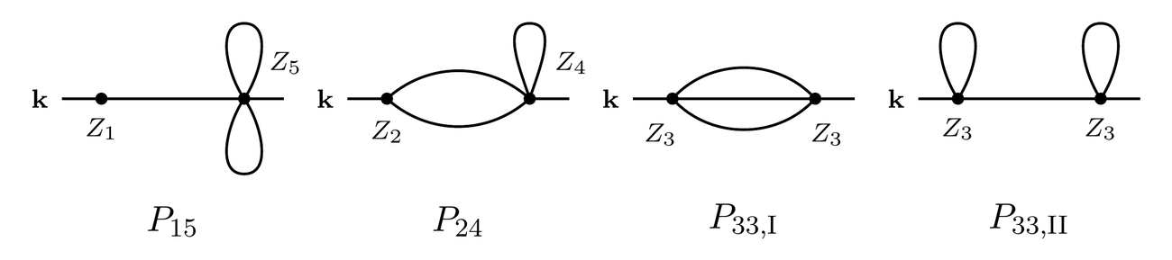
The four topologies of the two-loop galaxy power spectrum. Each dot is a redshift-space galaxy kernel $Z_n^{\rm gal}$, with the subscript giving its order, and each internal line is one linear power spectrum; a closed loop that begins and ends on the same dot is a pair of intermediate modes $(\mathbf{q},-\mathbf{q})$ contracted inside one kernel, a “tadpole.” In $P_{15}$ and $P_{33,\mathrm{II}}$ the line joining the two dots is not integrated over and gives an overall factor $P_{\rm lin}(k)$; $P_{33,\mathrm{I}}$ is the only topology without a tadpole. Filling the dots with pairs of bias and velocity coefficients gives 35, 42, 36 and 36 diagrams for the four topologies. (Figure 1 of Paper I.)
The hard part is evaluating the diagrams, because the terms cancel strongly: long-wavelength (soft) contributions cancel between diagrams, short-wavelength (ultraviolet) pieces cancel against counterterms, and inside one diagram the kernel is a sum of individually huge terms of alternating sign. For one matter kernel expanded in monomials the authors measure a cancellation by a factor of $1.3\times10^{17}$, more digits than double-precision arithmetic holds. The authors therefore integrate each diagram’s summed kernel directly and evaluate every tabulated component twice, in double and in extended precision. The two must agree to one part in a million; a component that misses this is re-evaluated, or its measured round-off is added to its stated error. Expanded in power laws, the pure matter integrands reduce to a two-loop master integral of particle physics called the kite. Paper I restates, from earlier notes by one of the authors, the closed form of the one kite family that lacked one; the derivation and its numerical checks are in its supplement.
The largest bare tables, meaning tabulated components before any subtraction, are those in which both loops close on themselves at composite bias operators. Most of each is a contact term, a piece with the shape of a lower-order term, which the renormalization conditions on the lower-order bias parameters remove. A counterterm basis that Paper I lists in full, though not yet reduced to a minimal independent set, absorbs the remaining ultraviolet sensitivity, whose leading shape is $k^2 P_{\rm lin}(k)$. The finite part of each table is then fixed by one of two linear maps on the tables; in the pivot condition, the subtracted table must vanish at $k_* = 0.2\,h\,{\rm Mpc}^{-1}$, which moves a $k^2 P_{\rm lin}$-shaped piece out of the table and into the counterterm coefficient.
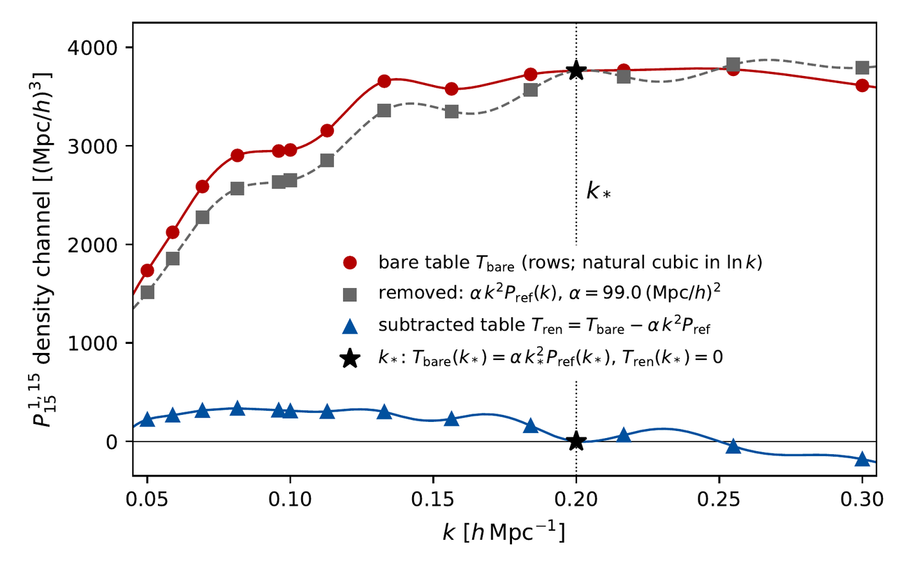
The pivot subtraction on one two-loop table, the density channel of one $P_{15}$ diagram (the linear bias $b_1$ paired with the fifth-order coefficient $\gamma_{41}$) at redshift 0.61. The bare table (red circles) is dominated by a piece with the counterterm’s shape $k^2 P_{\rm ref}(k)$ (gray squares, coefficient $\alpha = 99.0\,({\rm Mpc}/h)^2$); subtracting it so that the result vanishes at $k_* = 0.2\,h\,{\rm Mpc}^{-1}$ leaves the blue triangles, an order of magnitude smaller. The small wiggle of the blue curve near $k_*$ is the acoustic oscillation of $P_{\rm ref}$, which the smooth two-loop table does not share. Most of this bare table has the counterterm’s shape, and only the subtracted remainder is a prediction. (Figure 3 of Paper I.)
The infrared resummation is extended to two loops with the damping of the acoustic feature matched to the loop order: the linear, one-loop and two-loop oscillatory parts are damped by $e^{-x}(1+x+x^2/2)$, $e^{-x}(1+x)$ and $e^{-x}$, with $x = k^2\Sigma^2_{\rm tot}$. Here $\Sigma_{\rm tot}$ is the typical relative displacement of two points one acoustic scale apart, computed from the smooth linear spectrum rather than fitted. The one-loop damping acts inside the loop integrals.
By the same methods the authors compute the one-loop bispectrum. It has four loop topologies and 568 coefficient functions, the loop integrals that multiply each product of bias and velocity coefficients; the authors integrate them on a grid of 786 triangles. The bispectrum model has 17 counterterm coefficients and 19 stochastic parameters, three of the latter shared with the power spectrum. The authors organize the one-loop trispectrum into nine contraction types with up to 5209 coefficient functions, four families of counterterm insertions (one of them containing the fifteen cubic counterterm operators) and five further stochastic parameters. They evaluate all nine types on the 2400 parallelogram configurations that enter the covariance of the power spectrum. The figure below shows the sizes of the four bispectrum topologies before renormalization at a fiducial set of bias values. The two with a tadpole (a self-loop on one vertex) are a hundred times larger than the others at small $k$, where about 99 percent of each is a contact term. Renormalization absorbs that part into lower-order bias coefficients.
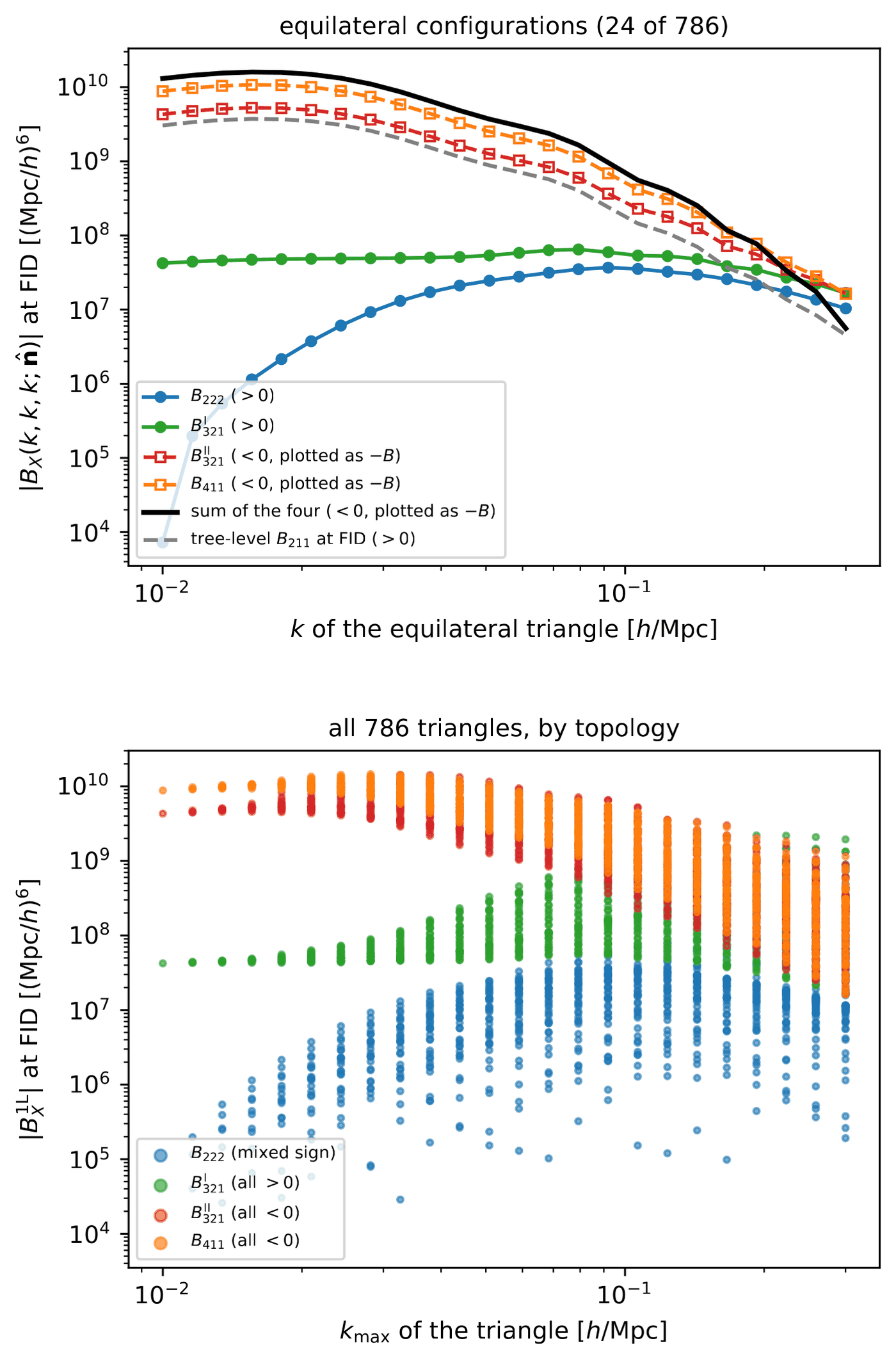
The four one-loop bispectrum topologies at Paper I’s fiducial bias point, contracted with the redshift-0.61 linear spectrum on the paper’s triangle grid: top, the equilateral triangles; bottom, every triangle against its longest side. Filled symbols are positive and open symbols negative values plotted as $-B$; the black line is the sum of the four and the gray dashed line the leading-order (tree-level) bispectrum. These are unsubtracted kernel integrals with no counterterms: the hundredfold dominance of $B_{411}$ and $B_{321,\mathrm{II}}$ at small $k$ is the contact term that renormalization absorbs into the lower-order bias coefficients, and by $k=0.3$ the four are within a factor 1.7 of one another with a sum one third of the largest (values given in Paper I’s supplement). The $B_{411}$ points predate a sign correction in one kernel that changes the norms of three of its 102 shape rows by at most 6 percent. The grid extends past the reach of the expansion: values at $k\gtrsim0.2\,h\,{\rm Mpc}^{-1}$ lie beyond its range of validity and say nothing about its accuracy. (Figure 5 of Paper I.)
The authors state what is unfinished in Paper I: five of the nine trispectrum types, computed so far only on those covariance configurations, remain to be evaluated on general quadrilaterals; six two-loop diagrams are listed but not assembled; and 31 velocity-dependent components of four further diagrams are not yet evaluated. The paper therefore shows no assembled, resummed two-loop curve and makes no comparison with simulations. The authors also stress that the two-loop term does not extend the reach of the expansion, which ends near $k \approx 0.2\,h\,{\rm Mpc}^{-1}$, where random galaxy motions along the line of sight become nonperturbative at any loop order. The two-loop term reduces the theoretical error inside that range; over $k \simeq 0.1$ to $0.2\,h\,{\rm Mpc}^{-1}$ the paper’s rough estimate puts the loop terms at a tenth to a fifth of $P$.
Paper II: the KITE code
Full-shape analyses today rely on public one-loop codes such as CLASS-PT, PyBird and velocileptors, which evaluate the one-loop power spectrum anew at every cosmology a sampler visits. A two-loop integral is too slow for that, and the bispectrum and trispectrum add many more nuisance parameters. KITE, the Kernel-Integral Tensor Engine of Paper II, therefore evaluates no loop integral while the likelihood runs. Every perturbative ingredient is a table computed once, the integral of the kernels against fixed basis functions for the linear spectrum, independent of cosmology. A sampled cosmology enters only through its expansion coefficients on that basis, and the prediction is a contraction of stored tables; renormalization, infrared resummation and the remapping of distances to the sampled cosmology are linear operations on them. All three statistics of Paper I are evaluated this way; the one-loop trispectrum tables are not yet complete, and every fit and test in this version of Paper II uses the tree (leading-order) trispectrum.
Each table entry is stored with its stated numerical error, and the authors give the linear map from table errors to shifts of the inferred parameters. The authors require that no single ingredient shift any parameter by more than $0.1\sigma$ or change any error bar by more than 5 percent, with all ingredients together held to $0.2\sigma$. So far the propagation covers the two-loop power spectrum tables of one redshift bin: the worst case is $0.2954\,\sigma$ or $0.1069\,\sigma$ depending on the data covariance, outside the single-ingredient allowance, and the authors claim no margin.
The fit to the power spectrum and bispectrum in six redshift bins samples 36 coordinates, the cosmological parameters plus a set of bias and shot-noise parameters for each bin. Another 384 parameters (bias combinations, counterterms, stochastic amplitudes) enter the model linearly, and KITE integrates them out in closed form. With $d_{\rm eff}$ the data residual after the nonlinear pieces are subtracted, in units of its noise (whitened), $J$ the matrix whose columns are the linear templates and $\Sigma$ the prior covariance of their coefficients,
$$M=\Sigma^{-1}+J^{\sf T}J\,,\qquad \hat x=M^{-1}J^{\sf T}d_{\rm eff}\,,\qquad \ln\mathcal L_P=-\tfrac12\big|J\hat x-d_{\rm eff}\big|^2-\tfrac12\,\hat x^{\sf T}\Sigma^{-1}\hat x-\tfrac12\ln\det M-\tfrac12\ln\det\Sigma\,.$$Here $\hat x$ is the best-fit value of the linear parameters at the current cosmology, the first two terms are the remaining misfit and the prior penalty on $\hat x$, and $-\tfrac12\ln\det M$ is the prior-volume termthe factor left behind when nuisance parameters are integrated out analytically; it depends on the cosmology and displaces the marginal posterior of amplitude-like parameters such as the primordial amplitude and sigma-8 from the peak of the full posterior, so it has to be tracked explicitly. Because it depends on the cosmology through $J$, the authors keep it explicit and report posterior means rather than maxima. The stochastic terms of the bispectrum are passed through the survey window, the imprint of the survey’s footprint and selection on every measured statistic, exactly as the data are. The remaining parameters are sampled by delayed-acceptance Hamiltonian Monte Carlo: trajectories and a first acceptance test use a fast, differentiable approximation to the linear spectrum, and a second test calls the Boltzmann code, at most once per chain per sweep (one trajectory for every chain). By construction the chains sample the exact posterior, and the approximation affects only the acceptance rate.
Tests on simulated data, and what is open
The authors test KITE on simulated data only, against acceptance conditions fixed before each fit, with a few stated exceptions. Synthetic data generated from the model itself, with a planted truth, test whether the fit recovers that truth (those fits are still running). A planted smooth bispectrum tests the window treatment (recovered on all six redshift blocks). Control catalogs of known content test the trispectrum estimator and template with the tree term of the model: eight configurations, no substantive failure, though most lacked the resolution to decide every test. The PT challenge simulations, a public code comparison, provide an external test (its parameters were disclosed to the participating teams in 2020, one of the authors among them, so the truth was withheld at the file level only, not from the people); the scale-cut sequence tabulated in this version comes from an earlier configuration and is kept as an illustration, with no final number quoted. A sampling run repeated with the same seed on two processor vendors reproduced its state bitwise at every checkpoint.
The $N$-body test of the joint likelihood uses a light-cone mock from the public AbacusSummit simulation suite: the mean of 25 simulated catalogs cut to the survey footprint, fitted jointly in the power spectrum and bispectrum over six redshift blocks with the covariance of a single catalog. The authors ran the fit twice, changing the treatment of the bispectrum’s stochastic rows. With the analytic rows, kept as a control, an excess in the mock bispectrum pushed the primordial amplitude $\ln 10^{10}A_s$ to the edge of its prior. With the rows imaged through the window, the bispectrum $\chi^2$ per row falls from between 0.56 and 0.96 to between 0.06 and 0.11 on all six blocks, and the amplitude moves off the prior boundary. Under a comparison rule fixed before that fit, four of five parameters designated beforehand then have posterior means within one posterior standard deviation of the simulation truth, and none beyond two (figure below). The exception is the cold-dark-matter density $\omega_{\rm cdm}$, low by 1.86 standard deviations, which the authors attribute to a residual on the power-spectrum side and not to the bispectrum. Two of the four clear the line by less than $0.1\sigma$, against a Monte Carlo error on the means of 0.03 to $0.05\sigma$, so the count of four holds only by that margin.
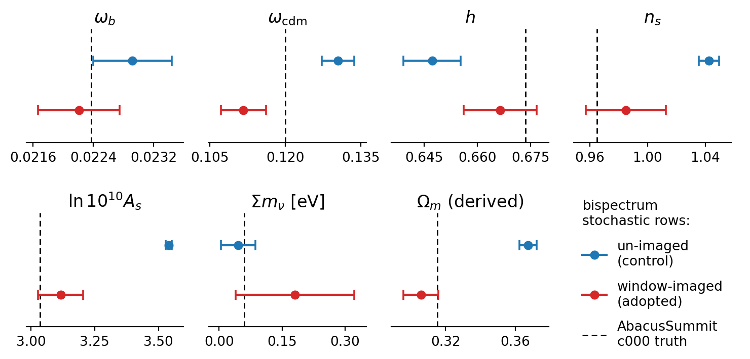
The joint power spectrum and bispectrum fit to the AbacusSummit light-cone mock, one panel per cosmological parameter: posterior mean and standard deviation with the analytic (un-imaged) stochastic rows, a control (upper point, blue), and with the window-imaged rows, the adopted treatment (lower point, red), against the simulation truth (dashed line). The widths are those of a single survey realization. Imaging the stochastic rows through the window moves $\ln 10^{10}A_s$ off its prior boundary and brings four of the five designated parameters ($\Omega_m$, $\ln 10^{10}A_s$, $h$ and $n_s$, but not $\omega_{\rm cdm}$) within one standard deviation of the truth; none of the five is within the $0.4\sigma$ benchmark adopted for survey use. (Figure 1 of Paper II.)
The window-imaged fit thus removes the control’s offsets, but it falls short of the tighter benchmark the authors adopt for applying the likelihood to survey data, recovery of the mock truth at the $0.4\sigma$ level: the five offsets range from 0.70 to 1.86 posterior standard deviations. The dedicated benchmark runs and the planted-truth fits are in progress and not reported in this preliminary version. No measurement from survey data and no cosmological conclusion appears in either paper.
The papers
- The loop expansion of galaxy clustering in redshift space — Matthew D. Schwartz, Mikhail M. Ivanov and Siddharth Mishra-Sharma; Paper I, in preparation; not yet posted, pending the co-authors’ approval. The authors derive the two-loop power spectrum, one-loop bispectrum and one-loop trispectrum of biased tracers in redshift space in one scheme, and state the numerical error of every loop integral evaluated so far.
- Supplementary Information for Paper I (with the paper, not yet posted) — the explicit kernels, the enumeration diagram by diagram, the full list of evaluated tables with their errors, and the derivation and numerical checks of the kite closed form that Paper I restates as Eq. (5.4).
- KITE: a two-loop galaxy clustering pipeline at stated precision — the same three authors; Paper II, in preparation; not yet posted, pending the co-authors’ approval. The authors describe the KITE likelihood code, its tables, error propagation, marginal likelihood and sampler, and its tests on simulated data.
- Supplementary Information for Paper II (with the paper, not yet posted) — the full list of tables, the longer derivations and the run-control details.
All three papers are in preparation and none is posted yet: the first drafts of Papers I and II were written by Claude (Anthropic), the text and computations are under review by the authors, each paper marks its unfinished items, and the third, on fits to survey data, is being written.
Supplementary material
Files hosted on this site. The script reproduces one check from Paper I. The machine-readable tables of the evaluated loop integrals are not yet posted; both papers state that the tables will be released with their final versions.
- lss-evaluate.py — a standalone Python script, needing only mpmath, that codes the closed form of the non-adjacent kite family as Paper I restates it in Eq. (5.4) and evaluates $K(1,\nu_2,\nu_3,1,\nu_5)$ at the paper’s first test point ($\nu_2 = 3/5 + 21i/100$, $\nu_3 = 9/20 - 33i/100$, $\nu_5 = 2/5 + 17i/100$), where Paper I’s supplement (Sec. S3) quotes $K = 0.0123418383\ldots + 0.0005742931\ldots\,i$. It compares the result digit by digit with the reference value in lss-reference-B1.json (next item) and runs in a few minutes; its
--checkoption adds an integer-relation test of that reference against the pieces of the closed form. - lss-reference-B1.json — the reference value of $K$ at that test point to 307 digits, computed by a different organization of the defining series and read by lss-evaluate.py.
References
| M. H. Goroff, B. Grinstein, S.-J. Rey and M. B. Wise, Coupling of modes of cosmological mass density fluctuations, Astrophys. J. 311 (1986) 6 | the recursion for the perturbative kernels $F_n$ of the matter density |
| N. Kaiser, Clustering in real space and in redshift space, Mon. Not. Roy. Astron. Soc. 227 (1987) 1 | the leading redshift-space distortion from galaxy velocities |
| P. McDonald and A. Roy, Clustering of dark matter tracers: generalizing bias for the coming era of precision LSS, JCAP 08 (2009) 020 | the general bias expansion relating the galaxy density to the matter density |
| D. Baumann, A. Nicolis, L. Senatore and M. Zaldarriaga, Cosmological non-linearities as an effective fluid, JCAP 07 (2012) 051 | recast the loop expansion as an effective field theory with counterterms |
| J. J. M. Carrasco, M. P. Hertzberg and L. Senatore, The effective field theory of cosmological large scale structures, JHEP 09 (2012) 082 | the effective field theory of large-scale structure, with counterterm coefficients fitted to data |
| J. J. M. Carrasco, S. Foreman, D. Green and L. Senatore, The Effective Field Theory of Large Scale Structures at two loops, JCAP 07 (2014) 057 | the two-loop matter power spectrum in the effective theory, in real space |
| L. Senatore and M. Zaldarriaga, The IR-resummed Effective Field Theory of Large Scale Structures, JCAP 02 (2015) 013 | resummation to all orders of the bulk flows that smear the acoustic feature |
| M. M. Ivanov and S. Sibiryakov, Infrared Resummation for Biased Tracers in Redshift Space, JCAP 07 (2018) 053 | the same resummation for galaxies in redshift space |
| A. Chudaykin, M. M. Ivanov, O. H. E. Philcox and M. Simonović, Nonlinear perturbation theory extension of the Boltzmann code CLASS, Phys. Rev. D 102 (2020) 063533 | CLASS-PT, one of the public one-loop codes used in the BOSS and DESI fits |
| G. D’Amico, L. Senatore and P. Zhang, Limits on wCDM from the EFTofLSS with the PyBird code, JCAP 01 (2021) 006 | PyBird, another of the public one-loop codes named beside CLASS-PT |
| S.-F. Chen, Z. Vlah and M. White, Consistent Modeling of Velocity Statistics and Redshift-Space Distortions in One-Loop Perturbation Theory, JCAP 07 (2020) 062 | velocileptors, the third public one-loop code named in Paper II |
| T. Nishimichi, G. D’Amico, M. M. Ivanov, L. Senatore, M. Simonović, M. Takada, M. Zaldarriaga and P. Zhang, Blinded challenge for precision cosmology with large-scale structure: results from effective field theory for the redshift-space galaxy power spectrum, Phys. Rev. D 102 (2020) 123541 | the PT challenge simulations that Paper II fits as an external test |
| N. A. Maksimova, L. H. Garrison, D. J. Eisenstein, B. Hadzhiyska, S. Bose and T. P. Satterthwaite, AbacusSummit: a massive set of high-accuracy, high-resolution N-body simulations, Mon. Not. Roy. Astron. Soc. 508 (2021) 4017 | the public simulation suite behind the light-cone mock of Paper II’s joint fit |
| P. Taule and M. Garny, The two-loop power spectrum in redshift space, JCAP 11 (2023) 078 | the two-loop matter spectrum in redshift space and its $k\approx0.2\,h\,{\rm Mpc}^{-1}$ limit |
| M. M. Ivanov, Galaxy Power Spectrum at Two-Loop Order: Implications for Weak Lensing Surveys and New Physics, arXiv:2606.30713 (2026) | the two-loop power spectrum of biased tracers in real space |
| T. Bakx, M. Garny, H. Rubira and Z. Vlah, Galaxy bias renormalization: Two-loop Power Spectrum, One-loop Trispectrum and Bispectrum, arXiv:2606.31280 (2026) | fifth-order bias renormalization of all three statistics, in real space |