Mixture models (statistics)
The content on this page was written by AI under human supervision.
A mixture model says that data come from several hidden subpopulations, and the oldest question asked of such data is how many there are. Among statisticians mixtures are notorious, “inherently evil” in one much-quoted verdict, and the Bayesian way to count subpopulations, comparing models by their evidence, rests on an integral long thought intractable for them. This paper computes the evidence exactly for mixtures of one discrete variable: at two subpopulations (components), at any number, and in the limit of infinitely many. The authors also show that ruling out a spurious subpopulation in a simple trial takes millions of participants, where the textbook criterion says twenty-two.
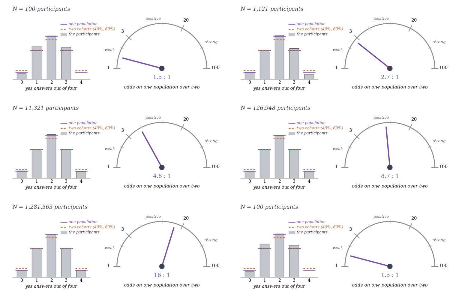
The paper’s running example as a tally. Each of $N$ trial participants answers yes or no four times; the bars show the fraction with 0 to 4 yes answers in one simulated trial where everyone answers yes half the time, the violet marks what one population predicts, the dashed orange marks an equal blend of two hidden cohorts answering yes 40 and 60 percent of the time. The dial gives the odds on one population against a model with two cohorts of any response rates, the Bayes factor, on the conventional scale where 3 counts as positive evidence and 20 as strong. Because the two-cohort model contains blends as close to one population as one likes, the odds grow only as the fourth root of $N$: the needle follows the paper’s large-sample law $0.46\,N^{1/4}$ for this design, which reaches 20 only near three and a half million participants (the exact odds, slightly above the law, cross 20 near $3.3$ million). (Illustration drawn for this page; the sample is simulated, the law is Corollary 2 of the paper.)
The twilight zone
In 1894 Karl Pearson fit a sum of two normal curves to Weldon’s crab measurements and asked whether the animals formed one population or two. His model is the prototype of a mixture model: each observation comes from one of $g$ hidden components, chosen with fixed probabilities called the weights, and each component has parameters of its own.
In August 2012 Larry Wasserman, a statistician at Carnegie Mellon University, put the case against mixtures on his blog Normal Deviate under the title “Mixture Models: The Twilight Zone of Statistics.” Mixtures are obviously useful, he allowed. He then listed what goes wrong in the simplest case, a mixture of bell curves, and closed: “I have decided that mixtures, like tequila, are inherently evil and should be avoided at all costs.” The post has been quoted and argued with ever since. Andrew Gelman replied eleven days later with a post of his own, “How I think about mixture models.” A 2016 paper by Feller, Greif, Miratrix and Pillai on weakly separated components first circulated as “Principal stratification in the Twilight Zone.” The model-selection chapter of the 2019 Handbook of Mixture Analysis, by Celeux, Frühwirth-Schnatter and Robert, ends by quoting the tequila verdict and declining to go that far. Matthew Schwartz and Subhabrata Sen, whose paper this page summarizes, quote the line in their introduction.
Wasserman’s seven items amount, in plain terms, to five complaints. First, the likelihoodthe probability of the observed data, read as a function of the model’s parameters; fitting usually means finding the parameters that make it largest misbehaves. For a mixture of bell curves it grows without limit as one component shrinks onto a single data point. Even where it stays finite it has many separate peaks, and the EM algorithm, the standard iterative fitting method, finds only one of them, depending on where it starts. Second, the components cannot always be told apart. Swapping two labels changes nothing, and, worse, wherever two components coincide or a weight is zero a parameter drops out of the model. Third, as a result, standard large-sample theory fails: likelihood-ratio tests and the Bayesian information criterion (BIC) assume a single well-behaved best fit, and even parameter estimates can converge unusually slowly.
Fourth, a flat priorthe probability distribution placed on a model’s parameters before seeing the data; a flat (improper) prior spreads evenly over an infinite range on a component’s location gives an improper posterior: the updated distribution of that location can never be normalized, at any sample size. A Bayesian must therefore commit to a proper prior, one that can itself be normalized. Fifth, fitted components need not mean what one hopes. A mixture of $g$ bell curves can have fewer or more than $g$ peaks, and assigning each point to its most probable component can carve up the data in unintuitive ways.
Two more difficulties, left aside in the post but spelled out in the paper’s introduction, concern the Bayesian route. A Bayesian compares one component against two through each model’s evidencethe marginal likelihood: the probability of the observed data under a model with its parameters averaged over their prior instead of set to best-fit values, and the ratio of two evidences is the Bayes factorthe factor by which the data multiply the prior odds between two models; by convention 3 counts as positive evidence and 20 as strong. For a mixture the evidence is an integral with $g^N$ terms at $N$ observations, one for each way of allocating observations to components. In practice it is estimated by Monte Carlo methods that have their own troubles here. Chib’s method, for one, falls short by $\log g!$ unless the simulation visits every relabeling of the components, the behavior called label switching.
Exact evidence for discrete data
Schwartz and Sen work with mixtures of one discrete variable. Each observation falls in one of $k$ cells, a dataset is summarized by the cell counts $U=(U_1,\ldots,U_k)$ of its $N$ observations, and each component is a vector of cell probabilities. The prior on each component is uniform or, more generally, Dirichlet, the standard family of priors on probability vectors. With whole-number Dirichlet parameters the two-component evidence is an explicit formula in the cell counts. Under uniform component priors the evidence is a finite sum at any number of components and in the infinite limit. The authors evaluate these sums exactly at sample sizes up to a hundred thousand, smaller as $g$ and $k$ grow (timings below). The input is a list of cell counts, the output one exact evidence per candidate number of components, and an implementation is linked at the end of this page. Nothing is simulated, so no error bar has to be taken on trust.
Of the five complaints, those about the likelihood vanish for discrete data: the likelihood is bounded, and since the evidence integrates over every parameter value, no peak has to be located and EM never runs. The label symmetry is integrated over with everything else. The deeper non-identifiability stays, because it belongs to the models. For one discrete variable it is total: a blend of $k$-cell distributions is again a $k$-cell distribution, and Teicher proved in 1963 that the components can then never be recovered from the data. So models with one, two or infinitely many components all describe the same set of distributions, and their evidences differ only through the priors that the component structure places on that set. The Bayes factor then compares priors rather than fits, and the exact values below show what that comparison comes to.
The third complaint also holds, since standard large-sample theory does fail for mixtures. Its correct replacement, Watanabe’s singular learning theory, fixes the rate at which the log evidence grows and leaves open a constant, which the authors supply for the trial design treated below and for two further discrete families. On the fourth complaint, every result uses proper priors, as the evidence integral requires, and each is stated for a specified range of priors, since the answers still depend on that choice. The authors do not take up the fifth complaint, about reading fitted components as clusters. They treat a mixture of two bell curves only in a large-sample idealization (below), so at finite sample size such mixtures stay where Wasserman left them.
The collapse of the sum
The computation rests on a cancellation. Multiplying out the two-component likelihood turns the evidence into a sum over all $2^N$ allocations of the observations to the components, each term a textbook integral in factorials. Evans, Gilula and Guttman wrote such sums down in 1989 and judged them too complicated for practical use. In 2009 Lin, Sturmfels and Xu reorganized them, proved that the evidence is a rational number, and evaluated it exactly for datasets of a few hundred observations. Schwartz and Sen notice that for one discrete variable the factorials from the likelihood cancel those from the component integrals. A term then depends only on how many observations went to the first component, whichever ones they are. The $2^N$ terms collapse to $N+1$, and partial fractions evaluate what remains in harmonic numbers, $H_j = 1+\tfrac12+\cdots+\tfrac1j$, which grow like $\log j$. For binary data with $n$ observations in each cell the two-component evidence under uniform priors is (Theorem 1)
$$Z(n,n) \;=\; \frac{(n!)^2}{(2n+1)!}\left[\frac{1}{n+1} + 2\big(H_{2n+1}-H_{n+1}\big)\right]$$
Here $Z(n,n)$ is the probability that the two-component model assigns to the observed data in the order recorded. Theorems 2 and 3 give the closed form for any counts, any number of cells and any whole-number Dirichlet priors. The one-component evidence at the same counts is the factor in front, $(n!)^2/(2n+1)!$, so the Bayes factor for one population against two is the reciprocal of the bracket at every $n$. Since $H_{2n+1}-H_{n+1}$ tends to $\log 2$, the Bayes factor tends to $1/(2\log 2)=0.72134\ldots$ (Corollary 1); it is already $0.7265$ at fifty observations per cell. A single yes-or-no variable split fifty-fifty thus never yields strong evidence either way, at any sample size, and the mild preference that remains favors the mixture. Away from fifty-fifty the limit is another constant, which favors one population only for splits more lopsided than about 20:80.
Components, readings and participants
Three whole numbers set the size of a mixture problem, the number of components $g$, of cells $k$ and of observations $N$, and the paper’s Table 6 sorts every application by them. At one extreme is the trial design below, with two components, five cells and millions of observations. At the other are two analyses from the supplement. Mutational signatures in cancer gene panels involve ten components and ninety-six cells but as few as five observations. In record linkage, which asks how many distinct individuals a file of noisy records refers to, the components are those individuals, and for the largest files analyzed they number in the tens of thousands.
The trial design that serves as the paper’s running example adds a fourth number, the readings $m$ per participant. A trial records a yes-or-no outcome $m$ times for each of $N$ participants, who thus fall into one of $k=m+1$ cells by their number of yes answers. If everyone responds with the same probability $\theta_0$ the expected counts are binomial; if the participants secretly form two cohorts, responders and non-responders, the counts follow a blend of two binomials, a little flatter (figure below).
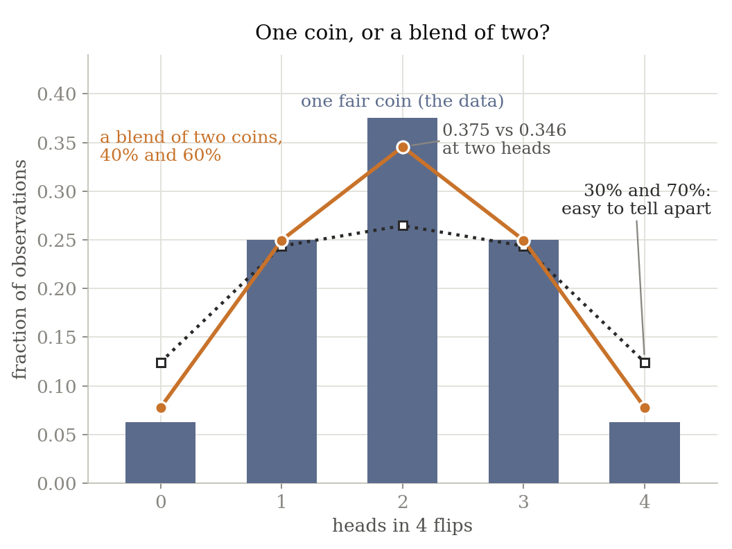
A mixture question in the four-reading design ($m=4$) used throughout the paper, drawn as coin flips (a head stands for a yes answer). Bars: the fraction of participants with 0 to 4 yes answers out of four when everyone responds with probability one half. Orange line: an equal blend of two cohorts responding with probabilities 0.4 and 0.6, which differs from the bars by three percentage points at two out of four. Dotted line: a blend of 0.3 and 0.7, visibly flatter. A mild blend is nearly indistinguishable from one population. (Illustration drawn for this page from elementary binomial probabilities; not a figure of the paper.)
Once each participant is read twice or more, one response probability fixes all of a cohort’s $m+1$ cell probabilities, whereas a component of the one-variable family above may have any cell probabilities at all. The two-cohort model therefore contains distributions that one cohort cannot produce, falls outside that family, and is not covered by the closed forms. The authors treat it through a large-sample expansion of its allocation sum, described next. The exact Bayes factors quoted below come from direct numerical integration over the model’s three parameters, the cohort weight and the two response probabilities. A trial designer wants to know how large $N$ must be, at given $m$, before the Bayes factor can favor one cohort ($g=1$) over a spurious second one ($g=2$) when one cohort is the truth.
With a single reading per participant ($m=1$), as shown above, no number of participants suffices. At $m=4$ the Bayes factor does grow with $N$, though slowly. In Watanabe’s theory the log evidence of each model falls below the best attainable log likelihood by $\lambda\log N$ plus a constant. The learning coefficient $\lambda$ is $1/2$ for one cohort and, by a 2004 result of Yamazaki and Watanabe, $3/4$ for the two-cohort binomial mixture. Schwartz and Sen obtain the missing constants on data with every count at its expected value. There the terms of the allocation sum peak along a whole ridge of ways to split the observations between the cohorts, and away from it their logarithm falls as the fourth power of the distance. Summing around the ridge gives the constant in closed form (Theorems 6 and 7). The Bayes factor for one cohort against two is then
$$\mathrm{BF}_{\,\rm ind:mix} \;=\; \frac{2\cdot 3^{1/4}}{\pi\,\Gamma(1/4)}\;\cdot\;\frac{N^{1/4}}{\sqrt{\theta_0(1-\theta_0)}}\;\big(1+o(1)\big)\,, \qquad \frac{2\cdot 3^{1/4}}{\pi\,\Gamma(1/4)} \;=\; 0.231089\ldots$$
where the subscript ind:mix means one population (the paper’s “independence model”) against the mixture, $\Gamma$ is Euler’s gamma function and $o(1)$ a correction that vanishes as $N$ grows (Corollary 2). The power $1/4$ is the difference of the two learning coefficients; the number in front comes from the ridge. Fourth-root growth is very slow: at $\theta_0=\tfrac12$ the exact Bayes factor first reaches 3, conventionally positive evidence, at $N=1{,}281$, and reaches 20, strong evidence, near $N=3.3$ million (figure below). BIC, the criterion most used in practice to choose the number of components, approximates each model’s evidence by dividing its best-fit likelihood by a factor of $\sqrt{N}$ for every free parameter. The mixture has two parameters more than a single cohort, so the BIC version of the Bayes factor grows in proportion to $N$. On the median dataset generated by one cohort it reports twenty-to-one odds against a second cohort already at $N=22$, where the true Bayes factor on expected-count data is about $1.2$: a gap of five orders of magnitude in sample size.
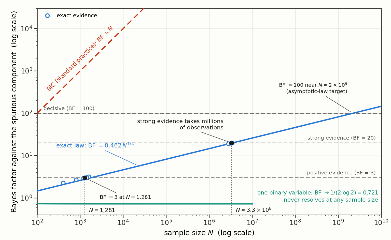
Bayes factor for one population against a two-component mixture with four readings per participant at a fifty-fifty response rate, on expected-count data, both axes logarithmic. Blue line: the asymptotic law above, $0.462\,N^{1/4}$ at $\theta_0=\tfrac12$; open circles: exact values; black dots: the crossings of 3 at $N=1{,}281$ and of 20 near $3.3$ million. Red dashes: the growth proportional to $N$ implied by a parameter-counting BIC. Teal: the single yes-or-no design, which converges to $1/(2\log 2)$ and never resolves. Strong evidence against a spurious component takes millions of observations, five orders of magnitude more than BIC suggests. (Figure 1 of the paper.)
The derivation goes through for any number of readings $m\ge 2$ and makes the trade-off between readings and participants explicit (equation (6.2) of the paper):
$$c_m(\theta_0) \;=\; \frac{\sqrt2\,\big(m(m-1)\big)^{1/4}}{\pi\,\Gamma(\tfrac14)\,\sqrt{\theta_0(1-\theta_0)}}\,, \qquad N^*(B) \;=\; \frac{B^4\,\pi^4\,\Gamma(\tfrac14)^4\,\big(\theta_0(1-\theta_0)\big)^{2}}{4\,m(m-1)}$$
Here $c_m(\theta_0)$ is the coefficient of $N^{1/4}$ in the Bayes factor, reducing at $m=4$ to the formula above, and $N^*(B)$ is the number of participants at which this asymptotic law reaches a target value $B$. The exact Bayes factor crosses a little sooner than the law, at $1{,}281$ rather than $1{,}775$ for $B=3$ above. The target enters as $B^4$, so asking for odds of 20 instead of 3 multiplies the enrollment by $(20/3)^4$, nearly two thousand. The readings enter as $1/(m(m-1))$, infinite at $m=1$, the never-resolving case, and equal to $1/2$, $1/12$ and $1/90$ at two, four and ten readings. Reading each participant ten times instead of four therefore divides the required enrollment by $7.5$. The factor $m(m-1)$ counts pairs of readings on one participant: hidden cohorts change how often the same person answers yes twice, and a single reading has no pairs to count. BIC, by contrast, reaches twenty-to-one at about twenty participants ($22$ in the four-reading case above) whether each is read once, four times or ten.
A mixture of two bell curves of known width obeys the same fourth-power law in the paper’s large-sample idealization (Proposition 1). With standard normal priors centered on the truth, the leading-order Bayes factor for one component reaches 3 near $8{,}600$ observations and 20 near $17$ million. All of these sample sizes are design values, for idealized data with every count at its expected value and for the stated priors, uniform ones in the trial design. Sampling noise moves the constant by a factor of order one, and a different prior moves it too; neither changes the fourth-root rate.
Any number of components, and infinitely many
The cancellation behind the two-component closed forms persists at any number of components $g$, provided the component priors are uniform (Theorem 4). A term then depends only on the $g$ component sizes, and the allocations with given sizes are counted by a classical generating function for contingency tables, whole-number arrays with fixed row and column totals. The resulting identity for the $g$-component evidence appears to be new.
The computing time depends on all three of the numbers $g$, $k$ and $N$, which trade off against one another. After the collapse the two-component evidence takes time polynomial in $k$ and $N$: Table 1 of the paper reports a thousand cells and $N=10^5$ in five minutes on one processor core, the answer an exact fraction. At general $g$ the work is governed by the smaller of $N^{g-1}$ and $N^k$. With many cells each further component costs roughly another factor of $N$ in time, and three components on 30 cells at $N=10^4$ take 19.4 minutes. With few cells the number of components all but stops mattering, and a million components on two cells at $N=5{,}000$ take 31 seconds (in floating point, checked against exact values at smaller sizes).
The modern way to avoid choosing $g$ is to make it infinite. Give the weights a symmetric Dirichlet prior with parameter $\alpha/g$ in each coordinate and let $g\to\infty$ at a fixed concentration $\alpha$; the limit is the Dirichlet processFerguson’s random probability distribution; as a prior over mixtures it lets the data fill as many clusters as they support, more readily at larger concentration mixture. Its evidence is a sum over every partition of the observations into clusters, some $10^{115}$ terms at $N=100$, and exact computations had reached about twenty observations. Theorem 5 takes the limit exactly. With the $\alpha/g$ weights the $g$-component evidence is a polynomial in $1/g$ of degree at most $N-1$, because an empty component contributes a factor of exactly one. Its constant term is the Dirichlet-process evidence, a finite sum over cluster sizes weighted by the same table counts, and passing to infinitely many components is the substitution $1/g=0$. On two cells the infinite case takes 79 seconds at $N=5{,}000$.
The authors evaluate the Dirichlet-process evidence on a standard test case, Escobar and West’s counts of eyetracking anomalies in 101 patients with schizophrenia, a computation done before only by Monte Carlo. The counts are binned into two or three cells; unbinned, on 35 cells, they are beyond the method’s reach. At seven concentrations from $1/3$ to $22/7\approx3.14$ the Dirichlet process is favored over its own truncations at one, two and three components every time, though never strongly: the $\log_{10}$ Bayes factors run from $0.04$ to $0.61$ (Table 5). The posterior on the number of occupied clusters, on the other hand, is driven by the concentration $\alpha$, a number the analyst chooses as part of the prior. The most probable cluster count moves from 2 to 12 across the grid, and the distribution is broad everywhere (figure below).
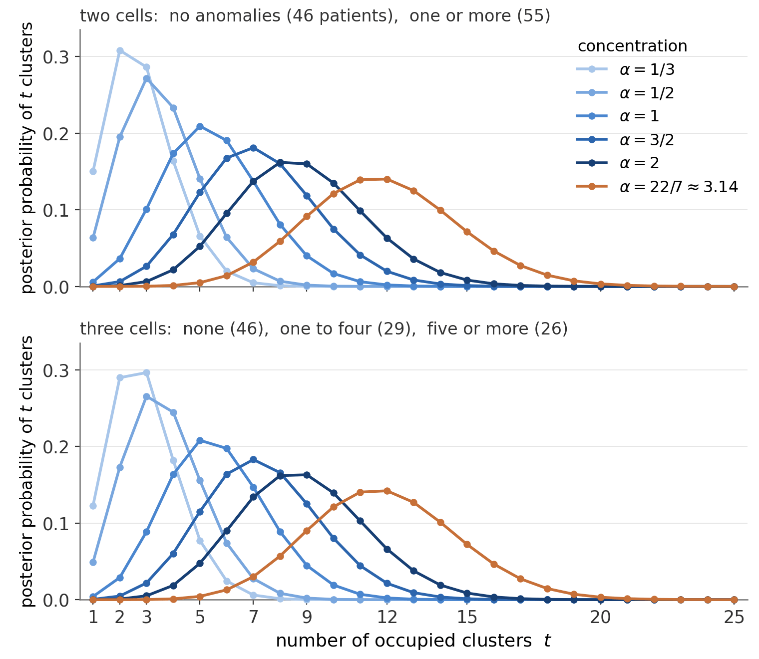
Exact posterior distribution of the number of occupied clusters for the Dirichlet process mixture on the eyetracking data ($N=101$ patients), under the two-cell binning (top: no anomalies, or at least one) and the three-cell binning (bottom: none, one to four, five or more), at six concentrations from $\alpha=1/3$ (lightest blue) to $\alpha=22/7$ (orange; the seventh grid value, $355/113$, gives a curve identical to it at this scale). As the concentration rises the most probable number of clusters moves from 2 (3 under the three-cell binning) to 12 and the distribution stays broad throughout: the data alone do little to fix the number of clusters. (Figure 2 of the paper, redrawn for this page from the same exact values.)
Checking the estimators
With exact values in hand one can also meet the complaint about Monte Carlo estimators directly, by measuring each estimator’s error instead of trusting its own error bar. The authors run five standard estimators at their default settings on the binary and binomial families (one reading and four readings per participant), at nine sample sizes from $N=100$ to $10^6$ with thirty simulated datasets each (Table 4). The harmonic mean is biased upward at every size, by $7.6$ nats (natural-log units) at $N=10^6$. Chib’s method diverges on the binomial family, with errors of order $10^6$ nats at $N=10^6$, and averaging over label permutations leaves the divergence in place, so label switching does not appear to be its cause. Bridge sampling agrees with the exact values up to $N\approx3{,}000$ and drifts low beyond, far short of the millions at which the trial question above is settled. Stepping-stone and nested sampling agree throughout, stepping-stone with a small downward drift (about half a nat) at $N=10^6$.
Limits and open problems
The collapse holds for one discrete variable only. Latent-class models, mixtures over several discrete variables at once, have no such reduction, and the authors report an analysis they could not finish. A two-class model for tuberculosis test data on 7,931 subjects would have needed a table of $1.32\times10^{14}$ entries, roughly a petabyte of memory. Beyond two components every exact value assumes uniform component priors. The large-sample constants are proved only for expected-count data, and how far the sample-size laws shift for randomly sampled counts is not settled in any family. For continuous components exact finite-sample evidence is out of reach beyond a handful of observations, since with continuous data the $g^N$ allocation terms are almost all distinct. For the bell-curve mixture, unknown widths and three or more components remain open even in the large-sample idealization.
The paper
- Exact Bayesian evidence for mixture models: from two components to infinity (PDF) — Matthew D. Schwartz and Subhabrata Sen; the version on this site is marked preliminary. Derives the closed forms and finite sums for the mixture evidence described above, the exact Dirichlet-process limit and the sample-size law for rejecting a spurious component, and compares the everyday Monte Carlo estimators with the exact values.
Supplementary material
Files and pages hosted on this site. The two Python scripts recompute exact values live and exit nonzero on any mismatch.
- Supplementary material (PDF) — the remaining proofs, including that of Theorem 6, the numerical methods and checks, the regime in which the number of states grows with the sample, and the six further applications summarized in Section 6.4 of the paper: capture–recapture, the Roman die count, the environmental-DNA survey, record linkage, the comparison of partition priors, and mutational signatures.
- Mixalot — the tool page on this site for the Mixalot package, which collects the paper’s exact-evidence evaluators behind one importable Python front door; usage, a capability map and worked examples.
- mixalot-package.tar.gz — the downloadable Mixalot bundle: the evidence engines (exact evidence as a rational number, the exact posterior on the number of components, the modular series route), each file checksum-pinned, with
mixalot.verify()failing if any pinned file has changed. - mixtures-evaluate.py — Python (mpmath): recomputes the numbers displayed on this page from scratch and compares them: the closed form $Z(n,n)$ for $n=1$ to $8$ against two independent allocation-sum engines, the coin-toss benchmark values of Lin, Sturmfels and Xu, and four closed-form constants, among them $1/(2\log 2)$ and $0.231089\ldots$, at two precisions. The
--fulloption adds the Bayes-factor values at $N=22$ and $N=1{,}281$ by direct quadrature, and--serieschecks the series files below. The default run takes a few seconds on a laptop;--fulladds under a minute. - lsx_direct.py — the standalone exact evaluator of the two-component allocation sum in rational arithmetic, with independent code paths cross-checked against the printed values of Lin, Sturmfels and Xu; the same file is included in the Mixalot bundle.
- series/SERIES_800.json — the exact evidence series $Z(n)$, $n=0$ to $800$, of the two-component binomial mixture in the four-outcome design along the ray $U=n\,(1,4,6,4,1)$, reduced modulo fourteen primes below $2^{25}$: the data behind the recurrence search of Section 4.5 of the paper and Section S3 of the supplement, which any proposed recurrence for this family must annihilate.
- series/ALLONES_SERIES_800.json — the same series along the all-ones ray $U=n\,(1,1,1,1,1)$, modulo two primes below $2^{24}$.
- series/README.md — the convention of the series files, how to check them (
python3 mixtures-evaluate.py --series, orsha256sum -c SHA256SUMS.txtinside the directory), the criterion by which they refute a claimed recurrence, and the route in the Mixalot bundle that regenerates or extends them.
References
| K. Pearson, III. Contributions to the mathematical theory of evolution, Phil. Trans. R. Soc. Lond. A 185 (1894) 71 | two normal curves fit to Weldon’s crab measurements; the first “one population or two” |
| H. Teicher, Identifiability of finite mixtures, Ann. Math. Statist. 34 (1963) 1265 | a mixture of one binary variable cannot be identified at any sample size |
| T. S. Ferguson, A Bayesian analysis of some nonparametric problems, Ann. Statist. 1 (1973) 209 | the Dirichlet process |
| G. Schwarz, Estimating the dimension of a model, Ann. Statist. 6 (1978) 461 | the BIC, a parameter-counting approximation whose assumptions mixtures violate |
| M. Evans, Z. Gilula and I. Guttman, Latent class analysis of two-way contingency tables by Bayesian methods, Biometrika 76 (1989) 557 | the mixture evidence as a finite sum, judged too complicated for practical use |
| R. E. Kass and A. E. Raftery, Bayes factors, J. Amer. Statist. Assoc. 90 (1995) 773 | the conventional scale on which a Bayes factor of 3 is positive evidence and 20 strong |
| S. Chib, Marginal likelihood from the Gibbs output, J. Amer. Statist. Assoc. 90 (1995) 1313 | Chib’s estimator of the evidence, one of the five tested against the exact values |
| S. Richardson and P. J. Green, On Bayesian analysis of mixtures with an unknown number of components, J. R. Stat. Soc. B 59 (1997) 731 | reversible-jump sampling of mixture posteriors with the number of components unknown |
| J. Pitman and M. Yor, The two-parameter Poisson–Dirichlet distribution derived from a stable subordinator, Ann. Probab. 25 (1997) 855 | the Pitman–Yor process, the two-parameter generalization of the Dirichlet process; one of the partition priors compared in the supplement’s record-linkage analysis |
| M. D. Escobar and M. West, Computing nonparametric hierarchical models, in Practical Nonparametric and Semiparametric Bayesian Statistics, Lecture Notes in Statistics 133, Springer (1998) 1 | the eyetracking data and their Monte Carlo analysis under a Dirichlet process mixture |
| K. Yamazaki and S. Watanabe, Newton diagram and stochastic complexity in mixture of binomial distributions, in Algorithmic Learning Theory, Lecture Notes in Computer Science 3244 (2004) 350 | the exponent $\lambda=3/4$ for the binomial mixture, without its constant |
| S. Watanabe, Algebraic Geometry and Statistical Learning Theory, Cambridge University Press (2009) | singular learning theory: the $\lambda\log N$ form of the log evidence for singular models |
| S. Lin, B. Sturmfels and Z. Xu, Marginal likelihood integrals for mixtures of independence models, J. Mach. Learn. Res. 10 (2009) 1611 | exact rational evidence for datasets of a few hundred observations; the family this paper builds on |
| L. Wasserman, Mixture models: the twilight zone of statistics, Normal Deviate (blog), August 4, 2012 | the list of mixture pathologies and the tequila verdict |
| Further reading for this page (not cited in the paper) | |
| A. Gelman, How I think about mixture models, Statistical Modeling, Causal Inference, and Social Science (blog), August 15, 2012 | the reply to Wasserman’s post, eleven days later |
| A. Feller, E. Greif, L. Miratrix and N. Pillai, Principal stratification in the Twilight Zone: weakly separated components in finite mixture models, arXiv:1602.06595 (2016) | weakly separated mixture components in causal inference; revised in 2019, with N. Ho, as Weak separation in mixture models and implications for principal stratification |
| G. Celeux, S. Frühwirth-Schnatter and C. P. Robert, Model selection for mixture models: perspectives and strategies, in Handbook of Mixture Analysis, S. Frühwirth-Schnatter, G. Celeux and C. P. Robert (eds.), Chapman and Hall/CRC (2019) 117 | chapter 7, on choosing the number of components, which closes by quoting the tequila verdict without going that far |